12 Decision Trees and the Random Forest Algorithm
This is a pre-release of the Open Access web version of Veridical Data Science. A print version of this book will be published by MIT Press in late 2024. This work and associated materials are subject to a Creative Commons CC-BY-NC-ND license.
The previous chapters have introduced algorithms, such as Least Squares (LS) and logistic regression, for generating predictions of continuous and binary responses. While these more traditional predictive algorithms are still commonly used in practice, the modern data science toolbox typically also contains several nonlinear predictive algorithms such as the Random Forest (RF) algorithm, which uses decision trees to generate predictions and will be the focus of this chapter. Other predictive algorithms that you are likely to encounter in your data science practice include Support Vector Machines, Kernel Ridge Regression, and Neural Networks (or “deep learning” algorithms);1 however, we won’t cover these in this book. See The Elements of Statistical Learning (Hastie, Friedman, and Tibshirani 2001) for a classic machine learning (ML) reference and Deep Learning (Goodfellow, Bengio, and Courville 2016) for a deep learning/neural networks reference.
12.1 Decision Trees
Have you ever used a flowchart that asked you a series of “yes” or “no” (i.e., binary thresholding) questions, eventually finding yourself funneled into one of several categories that lie at the end of a path through the tree? If so, then you’re already familiar with the basic ideas that underlie the decision tree-based algorithms that we will introduce in this chapter!
Just like a flowchart, a binary decision tree involves a series of binary questions arranged in a tree-like fashion. Each binary question involves asking either (1) whether the value of a continuous predictive feature is above or below a specific threshold value, such as “Did the user spend more than 20 minutes on product-related pages during their session?” (the continuous feature is the “product-related duration” and the threshold is 20), or (2) whether the value of a categorical predictive feature is equal to a specific level, such as “Did the session take place in December?” (where, for this example, the categorical feature is “month” and the level is “December”). Note that unlike the LS and logistic regression algorithms, algorithms that are based on decision trees can use categorical predictive features without requiring that they be converted to numeric (e.g., one-hot encoded dummy) variables.2
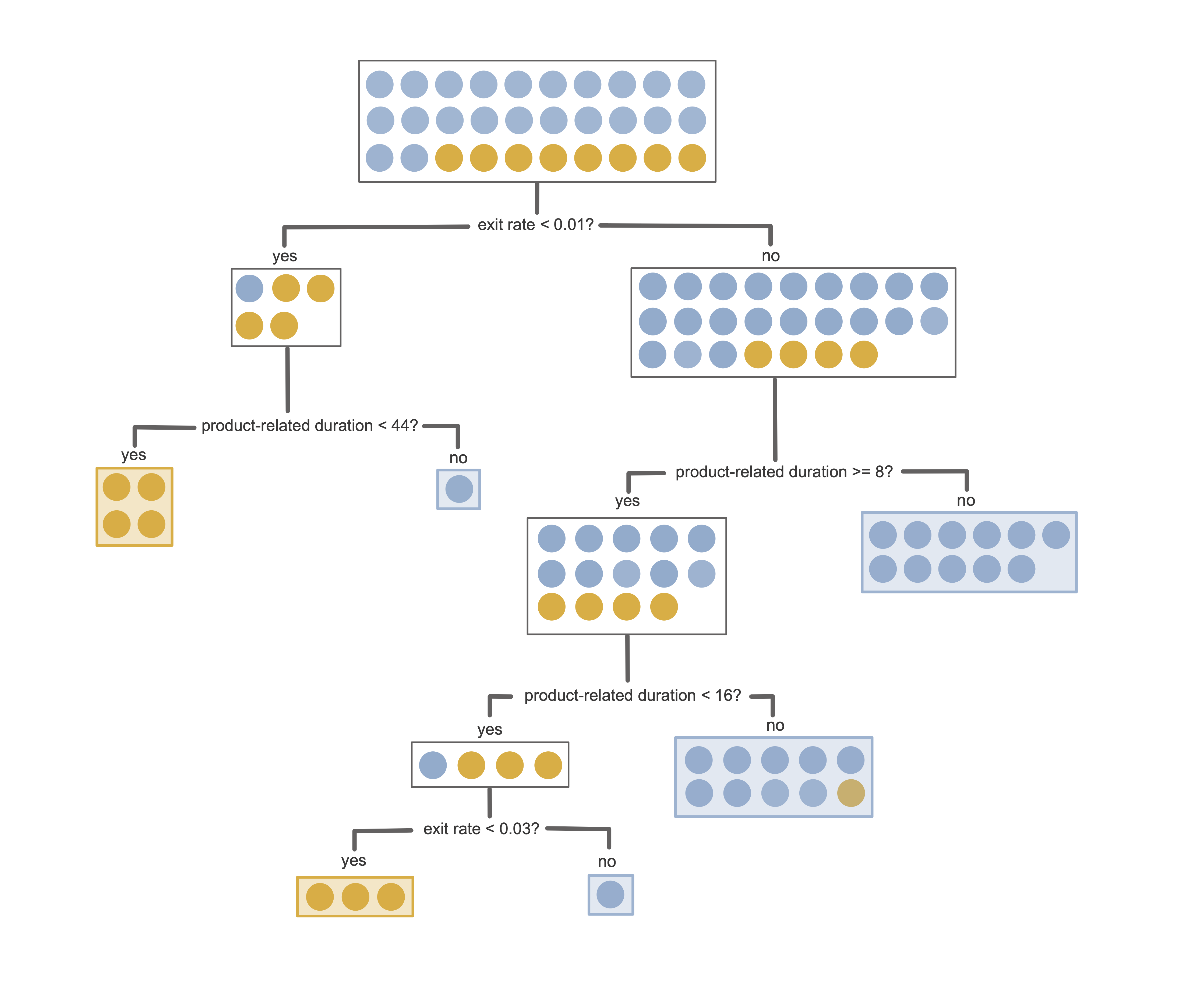
Figure 12.1 shows an example of a trained decision tree for predicting the purchase intent for the binary online shopping prediction problem introduced in Chapter 11. This decision tree involves just two features (exit rate and product-related duration in minutes) and was trained using a small sample of 30 training sessions (8 “positive class” sessions, which ended with a purchase, and 22 “negative class” sessions, which did not).
Let’s introduce some terminology: in our depiction of a decision tree in Figure 12.1, each rectangular box in the tree corresponds to a node that contains some subset of the training data. The node at the top of the tree contains the entire training set, which is sequentially split into pairs of child nodes (containing sequentially smaller and smaller subsets of the training data) according to binary (yes/no) questions. The nodes that lie at the end of a path (i.e., the nodes that are not split further) are called leaf nodes or terminal nodes, and it is in these leaf nodes where a binary or continuous response prediction is made. Note that for binary prediction problems, the leaf nodes don’t have to be pure—that is, they can contain observations from both classes (see Section 12.2.2).
Generating a response prediction for a new data point using a decision tree involves traversing through the tree for the new data point and identifying which leaf node it falls into. The response prediction for the new data point is then based on the set of training points that are in the corresponding leaf node. Unlike the LS algorithm, which was designed to predict continuous responses,3 and the logistic regression algorithm, which was designed to predict binary responses, decision trees can be used for both continuous and binary prediction problems.
For binary responses, a positive class probability response prediction (similar to the output of logistic regression) for a new data point can be computed based on the proportion of positive class training observations that are in the corresponding leaf node. A binary response prediction can then be computed using a thresholding value (just as for the logistic regression algorithm). The default threshold is 0.5, but when the number of observations in each class is imbalanced, it is often helpful to choose a threshold that corresponds to the proportion of observations that are in the positive class in the training data (which is 16.1 percent for the online shopping dataset). A continuous response prediction is usually based on the average response of the training observations in the corresponding leaf node.
For the decision tree in Figure 12.1 (where orange corresponds to “purchase” and blue corresponds to “no purchase”), can you predict the purchase intent for a new user session that spent 20 minutes on product-related pages and had an average exit rate of 0.042?
Probably the most powerful property of a decision tree lies in its interpretability and ease of use. The predictions produced by a (reasonably small) decision tree are very transparent: by following the path of a new data point through the tree, you can see exactly how each feature led to the resulting prediction. Moreover, you don’t even need a computer to produce a prediction for a new data point using a decision tree (assuming that the tree is simple enough that you can visually traverse through a diagrammatic depiction of it). For this reason, decision trees are often used in the medical field to generate simple clinical decision rules, which are used by clinicians in medical settings to make diagnoses and treatment decisions.
12.2 The Classification and Regression Trees Algorithm
Training a decision tree involves identifying the set of binary questions that minimize some relevant loss function. However, rather than aiming to minimize a loss for the final predictions generated by the decision tree, most decision tree algorithms aim to minimize a loss for each individual split. Algorithms that optimize a loss at each iteration (at each split, in this case), rather than optimizing the final results, are called greedy optimization algorithms.
12.2.1 Choosing the Splits
To determine what loss we should minimize at each split, let’s first think about what might make a “good” split question. A sensible goal would be to create nodes that consist of training observations whose responses are similar to one another, which means that we first need to define “similarity” in this context.
For continuous responses, a reasonable measure of the similarity between the responses of the data points in a node involves computing their variance. The smaller the variance of the responses, the more similar they are to one another. Thus, a reasonable split (e.g., one of exit rates < 0.05, exit rates < 0.024, or product type duration < 300) might be the one for which the responses of the data points in each of the resulting child nodes have the smallest variance.
For binary responses, computing the variance of the responses (that are each equal to either 0 or 1) yields a measure of the impurity of the training observations in the node. A pure node consists entirely of observations from just one class (rather than a mixture of the two classes). Thus, an equivalent goal for binary responses might be to choose a split (e.g., month = "June", month = "April", browser = "firefox", or browser = "safari") that produces child nodes that are maximally pure (or minimally impure).
The most popular binary decision tree algorithm, the Classification and Regression Tree (CART) algorithm (Breiman et al. 1984), works by computing the splits that minimize the variance of continuous responses or the impurity of the binary responses in each resulting child node. Although you generally won’t have to implement these computations yourself (because the rpart package in R and the scikit-learn library in Python, have functions/classes that will implement this algorithm for you), it is still helpful to understand how they work, so let’s dive a little deeper into the splitting measures that are used in the CART algorithm.
12.2.1.1 The Variance-Splitting Measure for Continuous Responses
As we have mentioned, for continuous response prediction problems, the CART algorithm chooses the split for which the responses in each child node will have minimum variance. Since this measure is a function of the two child nodes, and each node may have a different number of observations, computing this variance measure for a split involves computing a weighted combination of the variance across the left and right child nodes:
\[ \textrm{Variance measure for split} = \frac{n_\textrm{left}}{n_\textrm{parent}}\textrm{Var}_{\textrm{left}} + \frac{n_\textrm{right}}{n_\textrm{parent}}\textrm{Var}_\textrm{right}, \tag{12.1}\]
where \(n_\textrm{left}\) is the number of training observations in the left child node, \(n_\textrm{right}\) is the number of training observations in the right child node, \(n_\textrm{parent}\) is the number of training observations in the parent node, \(\textrm{Var}_{\textrm{left}}\) is the variance of the responses of the training observations in the left child node, and \(\textrm{Var}_{\textrm{right}}\) is the variance of the responses of the training observations in the right child node.
To demonstrate this variance split measure, let’s compute the first split of a decision tree for the Ames house price prediction project based on just two predictor variables (greater living area and neighborhood) for a sample of 30 houses from the Ames housing dataset. The CART algorithm works by identifying a range of plausible splits and computes the variance-splitting measure for each plausible split. Table 12.1 shows the value of the variance-splitting measure for several potential split options, in which the split “living area < 1,428” yields the lowest variance and is thus the split that is chosen. The code for this example can be found in the 06_prediction_rf.qmd (or .ipynb) file in the ames_houses/dslc_documentation/ subfolder of the supplementary GitHub repository.
| Split | Variance measure |
|---|---|
| living area < 1,625 | 1,343,422,176 |
| living area < 1,428 | 808,915,591 |
| living area < 905 | 1,255,484,629 |
| neighborhood = NAmes | 1,982,880,348 |
| neighborhood = CollgCr | 832,579,146 |
12.2.1.2 The Gini Impurity Splitting Measure for Binary Responses
The most common loss function for conducting a split for binary responses is called the Gini impurity, which turns out to be essentially equivalent to the variance measure that we just introduced for continuous responses. The Gini impurity of a split measures the impurity of the child nodes that are created by the split. In a pure node, all the observations are in the same class (i.e., each observation has the same binary response). In contrast, an impure node has a mixture of both classes. For example, if a split led to a child node with nine positive class observations and one negative class observation, then the node is fairly pure (since it is mostly positive class observations). In contrast, a node consisting of half positive and half negative class observations is maximally impure. Some split options will lead to child nodes that are more pure than others, and our goal is to find the split that leads to the most pure/least impure child nodes, as measured by the Gini impurity.
The Gini impurity of a set of observations is defined as the probability that two randomly chosen observations (where we are assuming that the two observations are sampled with replacement) from the node are in different classes (e.g., one is in the positive class and the other is in the negative class).
Using the statistical notation, \(P(x)\), for the probability that event \(x\) will happen, the Gini impurity can be written as
\[ \textrm{Gini impurity = }P(\textrm{two random obs in different classes}). \tag{12.2}\]
If all observations in the node were in the same class (i.e., the node is pure), the Gini impurity would equal 0, because the chance of randomly drawing two observations from different classes is 0. On the other hand, if the node were made up of equal numbers of observations from each class, the Gini impurity would equal 0.5 (since, after drawing one observation, the chance of the next random draw being an observation from the other class is 50 percent, assuming that we are drawing with replacement). Since we are trying to minimize node impurity, a lower Gini impurity is better.
Because the probability of any event occurring is equal to 1 minus the probability of the inverse of that event occurring, the Gini impurity can also be written as
\[ \textrm{Gini impurity} = 1 - P(\textrm{two random obs in the same class}). \tag{12.3}\]
Moreover, since the event that “both observations are in the same class” is equivalent to the event that “both observations are in the positive class OR both observations are in the negative class” (and since for two events, \(A\) and \(B\), we can write \(P(A \textrm{ or } B) = P(A) + P(B)\)), we can alternatively write the Gini impurity as
\[ \textrm{Gini impurity} = 1 - \Big(P(\textrm{both pos class}) + P(\textrm{both neg class})\Big), \tag{12.4}\]
where “both pos/neg class” means “two randomly selected observations are both in the positive/negative class.”
Why do we want to decompose the Gini impurity in this way? Our goal is to transform the Gini impurity into a format that is easier to compute. To see why this is easier to compute, let’s denote the probability that a single randomly selected observation is in the positive class as
\[ p_1 = P(\textrm{a randomly selected observation is in the positive class}). \tag{12.5}\]
This value, \(p_1\), is just equal to the proportion of the observations in the node that are in the positive class. Next, the probability that two randomly selected observations would be in the positive class (assuming that we are sampling with replacement) is equal to \(p_1 \times p_1 = p_1^2\).
If we similarly denote the probability of a randomly selected observation being in the negative class as \(p_0\), then plugging these values into Equation 12.4 leads to
\[ \textrm{Gini impurity} = 1 - p_1^2 - p_0^2, \tag{12.6}\]
where \(p_1\) and \(p_0\) are the proportion of the observations that are in the positive and negative classes, respectively. Note that if a binary variable is equal to 1 with probability \(p_1\) and is equal to 0 with probability \(p_0\), where \(p_0 +p_1 = 1\) (i.e., it has a Bernoulli distribution), then the variance of this binary variable can be shown to equal \(\textrm{Var} = p_0 p_1 = p_0(1 - p_0) = p_0 - p_0^2\), or equivalently, \(\textrm{Var} = p_0 p_1 = (1 - p_1)p_1 = p_1 - p_1^2\). Adding these two versions of the variance together returns the Gini impurity measure
\[ \begin{align} 2\textrm{Var} &= p_0p_1 + p_0p_1 \\ \nonumber & = (p_0 - p_0^2) + (p_1 - p_1^2)\\ \nonumber & = p_0 + p_1 - p_0^2 - p_1^2 \\ \nonumber & = 1 - p_0^2 - p_1^2\\ \nonumber & = \textrm{Gini impurity}, \nonumber \end{align} \tag{12.7}\]
which shows that minimizing the continuous response variance measure in the context of binary responses is the same as minimizing the Gini impurity!4
Let’s consider some examples. If a node contains an equal number of observations from each class, then \(p_1 = p_0 = 0.5\) and its Gini impurity is
\[\textrm{Gini impurity }= 1 - 0.5^2 - 0.5^2 = 0.5,\]
which is as impure as a set of observations can get. If we instead have 75 percent of the observations in one class and 25 percent in the other class, the Gini impurity is then equal to
\[\textrm{Gini impurity }= 1 - 0.25^2 - 0.75^2 = 0.375,\]
which is smaller than \(0.5\), indicating that this node is less impure (more pure). Note that the Gini impurity of the child nodes will always be less than the Gini impurity of the parent node (i.e., the child nodes are always more pure than the parent nodes).
To see the Gini impurity in action, let’s use it to evaluate the first split from the binary online purchase intent prediction problem decision tree from Figure 12.1. This first split, shown in Figure 12.2, involves asking if “exit rates < 0.01?”
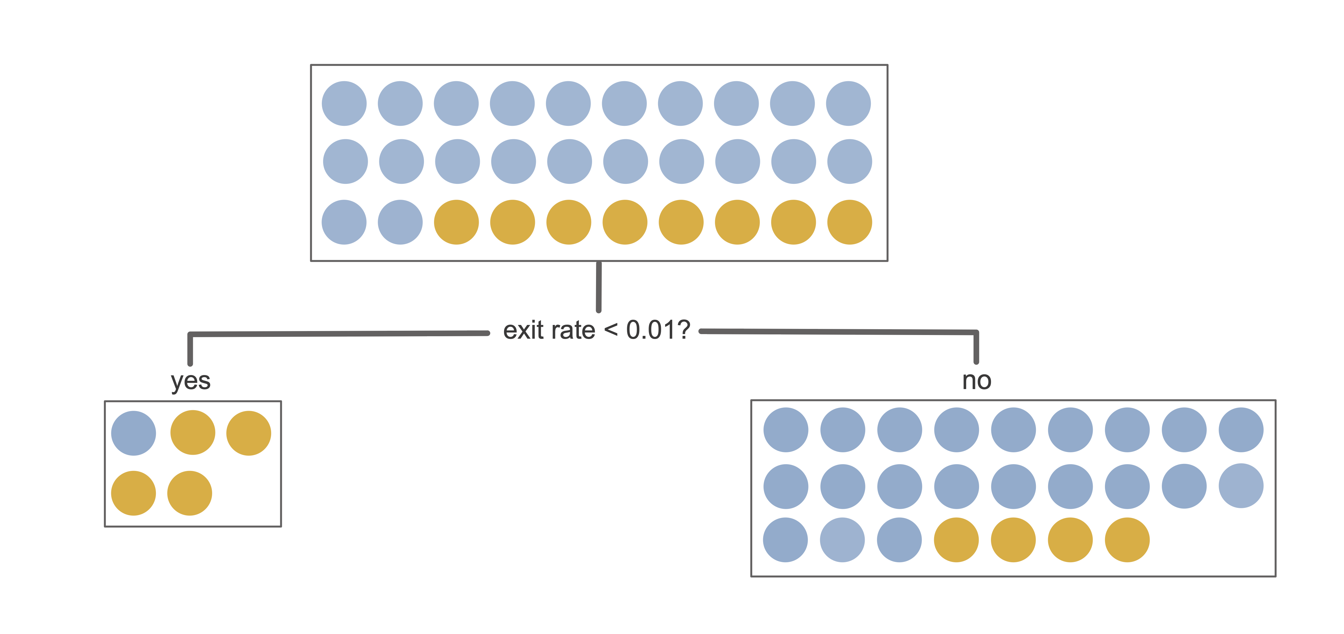
The left “yes” child node of this split contains five data points total, four of which are in the positive class and one of which is in the negative class. The Gini impurity of the left “yes” child node is thus
\[\textrm{Gini}_{\textrm{left}} = 1 - \left(\frac{4}{5}\right)^2 - \left(\frac{1}{5}\right)^2 = 0.32.\] Similarly, the Gini impurity of the right “no” child node is
\[\textrm{Gini}_{\textrm{right}} = 1 - \left(\frac{4}{25}\right)^2 - \left(\frac{21}{25}\right)^2 = 0.27.\]
To compute the Gini impurity of the entire split rather than just each individual child node, we need to combine the left- and right-child Gini impurity values. However, recall that each child node has a different number of observations, so to make sure that each observation is contributing to the overall Gini impurity equally, we can apply a weight to each of the child node Gini impurity values based on the number of observations that it contains (just as we did for the variance measure):
\[ \textrm{Gini impurity for split} = \frac{n_\textrm{left}}{n_\textrm{parent}} \textrm{Gini}_{\textrm{left}} +\frac{n_{\textrm{right}}}{n_{\textrm{parent}}}\textrm{Gini}_{\textrm{right}}, \tag{12.8}\]
So the Gini impurity for this first example split is
\[\textrm{Gini impurity for split} = \frac{5}{30} \times0.32 + \frac{25}{30} \times0.27 = 0.28.\]
To choose this particular split, the CART algorithm computed the Gini impurity for a range of possible split options and this was the one that yielded the lowest Gini impurity. Table 12.2 shows several possible binary thresholding options for this first split and the corresponding Gini impurity value (notice that the exit rates < 0.01 yields the lowest Gini impurity). If you want to try to compute these Gini impurity values for yourself, the code for creating the sample of 30 training houses and manually computing these variance-splitting measures can be found in the 04_prediction_rf.qmd (or .ipynb) file in the online_shopping/dslc_documentation/ subfolder of the supplementary GitHub repository.
| Split | Gini |
|---|---|
| exit_rates < 0.01 | 0.28 |
| exit_rates < 0.025 | 0.37 |
| exit_rates < 0.031 | 0.36 |
| product_related_duration < 8.41 | 0.31 |
| product_related_duration < 3.85 | 0.36 |
| product_related_duration < 15.92 | 0.39 |
12.2.2 Stopping Criteria and Hyperparameters
While it might seem sensible to continue to conduct splits until each child node is pure (i.e., all observations in the child node are in the same class), this can lead to unnecessarily deep trees (i.e., trees with a large number of sequential splits). It is therefore common to regularize the CART algorithm by implementing stopping criteria that limits the maximum depth of the tree (i.e., the number of sequential splits allowed) and/or do not allow splits of nodes with fewer than some minimum number of observations.
While the CART algorithm is very different from the lasso and ridge algorithms from Chapter 10, our use of the term “regularization” here has a very similar purpose: to limit the possible complexity of the fit produced by the algorithm. Recall that regularization can help prevent the algorithm from learning patterns that are too specific to the training data (overfitting), which can in turn help improve the stability of the resulting fit and help it generalize to new data. The two most important CART hyperparameters for regularization are listed in Box 12.3.
12.2.3 Generating Predictions
Recall that generating response predictions for a new data point using a decision tree involves identifying which leaf node the observation falls into and looking at the responses of the training data points in the leaf node. For binary response problems, there are two types of response predictions that you can generate:
Positive class probability prediction: The predicted positive class probability is the proportion of the training observations in the leaf node that are in the positive class.
Binary class prediction: A binary prediction can be computed using the “majority” class (the class that makes up at least 50 percent of the observations) of the training observations in the leaf node. For problems with class imbalance, it often makes more sense to instead use a threshold equal to the proportion of training set observations in the positive class (or tuned using CV).
Continuous response predictions can be computed using the average response of the training observations in the leaf node.
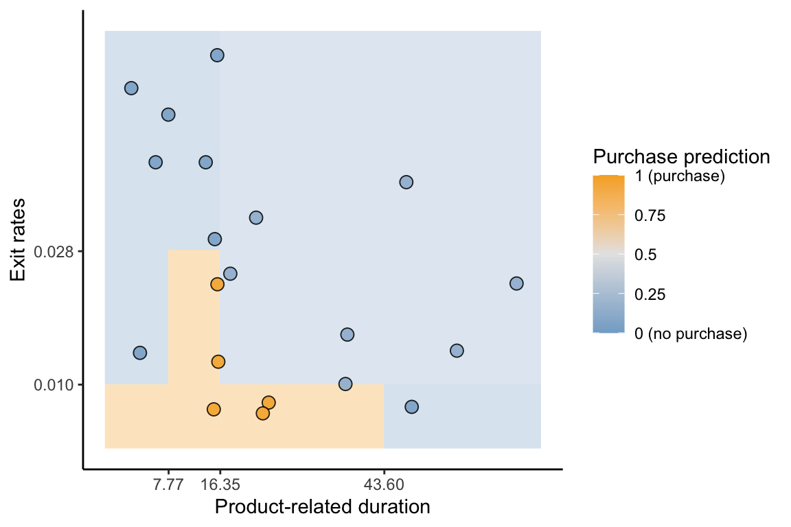
Figure 12.3 shows the decision boundary for the two-predictor (exit rates and product-related duration) CART algorithm for predicting the probability of a purchase based on the decision tree in Figure 12.1. The color of the background corresponds to the purchase (positive class) probability prediction for a new data point in that location. Each distinct rectangle corresponds to a split in the decision tree from Figure 12.1. Compare the CART classification boundary in Figure 12.3 to the logistic regression classification boundary in Figure 11.7 in Chapter 11. Unlike the logistic regression classification boundary, the CART decision boundary is made up of discrete blocks of constant positive class probability predictions.
A summary of the CART algorithm is provided in Box 12.4.
12.3 The Random Forest Algorithm
Although a single decision tree is simultaneously interpretable and computationally simple, this is typically (but not always) at the cost of predictive performance. This is particularly true for continuous response prediction problems: a decision tree with only 20 terminal leaf nodes can produce only 20 distinct response predictions, but most datasets with continuous responses will contain far more than 20 distinct response values!
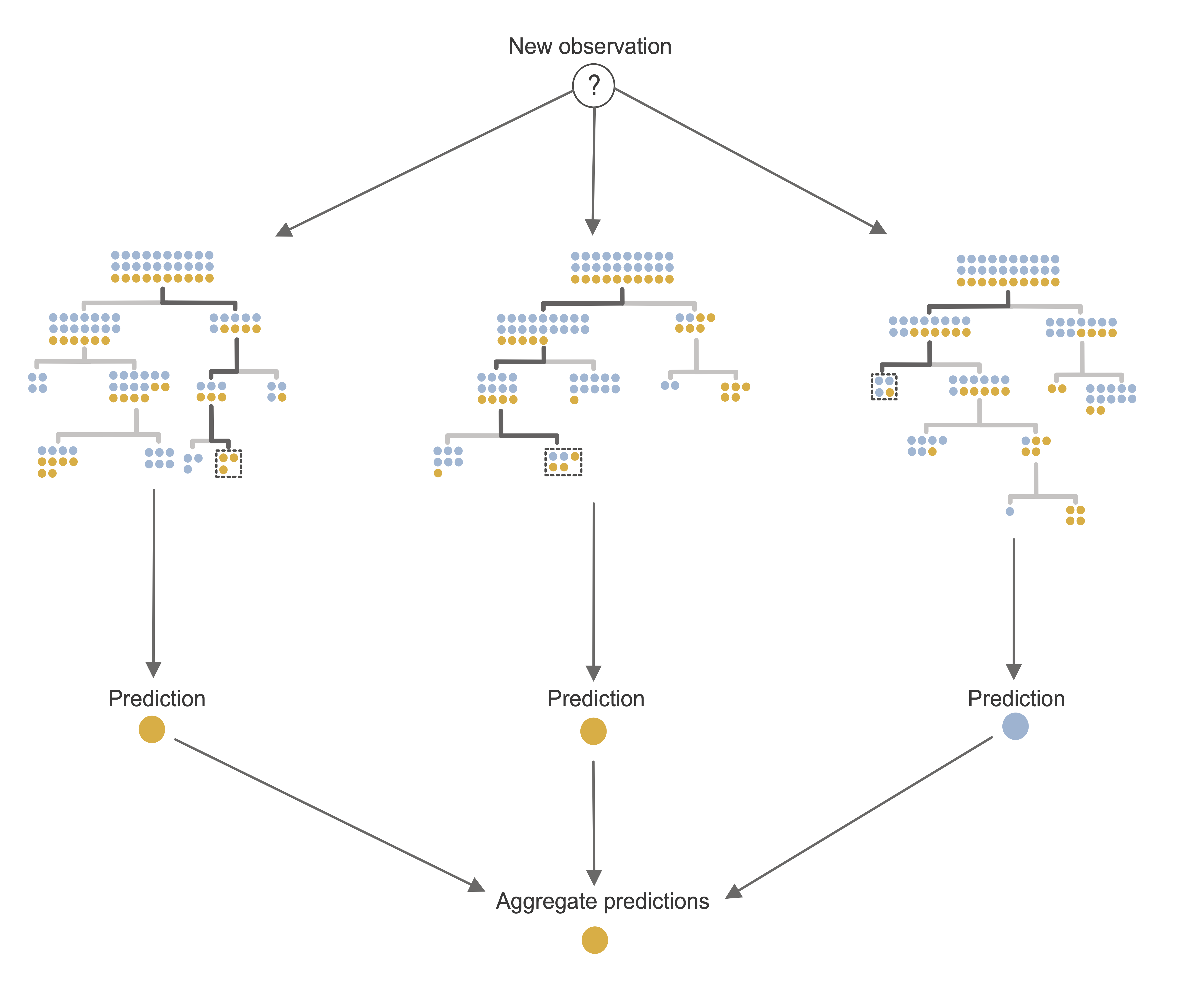
There are, however, several predictive algorithms that extend the CART algorithm specifically to address this issue. The primary example of this is the Random Forest (RF) algorithm (Breiman 2001). RF is an ensemble algorithm that works by aggregating the predictions computed across many different decision trees, thereby allowing a broader range of predicted response values to be computed than would be possible from a single decision tree.
Just as a real-world forest consists of many trees that are each similar to, but slightly different from one another, a random forest consists of many decision trees that are each similar to, but slightly different from one another. The RF algorithm does this by training each decision tree using a bootstrapped sample of the training data. Recall that a bootstrapped sample is a random sample of the same size as the original data, where the sampling is performed “with replacement”, which means that each observation may be included in the sample multiple times (or not at all). Additional randomness is introduced into each tree by considering a different random subset of the predictive features for each individual node split.
The end result is a collection of decision trees, each capturing a slightly different snapshot of the patterns and relationships in the training data. Intuitively, this means that it is more likely that such a forest-based algorithm will be able to generalize to new data that is slightly different from the training dataset. As a general principle, the more independent the trees are from one another, the more accurate and generalizable the RF ensemble predictions they generate will be (however, each tree must still be a reasonable representation of the original data).
Just as for the CART algorithm, there are two types of RF response predictions that you can compute for a binary response:
Positive class probability prediction:5 The average of the positive class probability predictions from the individual trees.
Binary class prediction: The majority vote of each of the individual tree’s binary predictions (or a thresholded version of the RF class probability prediction).
For continuous response prediction problems, a continuous response prediction can be computed as the average prediction across the individual trees.
A summary of the RF algorithm is provided in Box 12.5
An RF fit based on an ensemble of just three trees is depicted in Figure 12.4. A typical RF fit, however, will usually involve more like 500 trees.
While the original implementation of the RF algorithm in R is from the “randomForest” package (Breiman 2001), we typically use the “ranger” package (Wright and Ziegler 2017) due to improved computational speed. The scikit-learn Python library also has an implementation of the RF algorithm via the ensemble.RandomForestClassifier() class.
Note that RF fits are invariant to monotonic transformations of the underlying variables, meaning that applying logarithmic, square-root, and other variable transformations will not affect the resulting fit.
12.3.1 Tuning the RF Hyperparameters
Like the CART algorithm, there are many hyperparameters for the RF algorithm that can be tuned. The RF hyperparameters include the original CART hyperparameters, the depth of the tree, and the minimum node size for splitting, as well as several other hyperparameters, such as the number of trees in the forest ensemble and the number of randomly chosen variables to be considered at each split.6 These hyperparameters can be tuned using CV, but in general, we find that the default hyperparameters work quite well for most packages. A summary of the most important RF hyperparameters is shown in Box 12.6.
12.4 Random Forest Feature Importance Measures
Recall that the standardized LS and logistic regression feature coefficient values (where you can either standardize the input predictive features before fitting or standardize the coefficients themselves) can be used as a measure of feature importance for the predictive algorithm. Although there are no feature coefficients in an RF fit, the RF algorithm itself has a few built-in techniques for computing the importance of each feature, the two most common of which are (1) the permutation importance score and (2) the Gini importance score.
12.4.1 The Permutation Feature Importance Score
The permutation feature importance score for a single feature—let’s call it feature “\(x\)”—involves identifying how much the mean squared error (MSE; for continuous responses) or prediction accuracy (for binary responses) decreases when retraining the RF algorithm using a permuted (a permutation is a type of perturbation) version of \(x\) together with the original unpermuted versions of the other predictive features. Permuting a feature involves randomly shuffling the feature’s values across the training observations, which destroys any existing relationships between the feature and the response (as well as the other predictive features). If the predictive performance does not change when feature \(x\) is permuted, then feature \(x\) is unlikely to be a particularly important predictive feature. On the other hand, if permuting feature \(x\) results in a notable drop in predictive performance, this indicates that it was probably a particularly important predictive feature.
Note that the predictive performance that we compute when conducting permutation feature importance is based on the training data (rather than the withheld validation set or external data). However, rather than using the traditional training error (training and evaluating the algorithm both on the same training set), it is more common to compute the out of bag (OOB) prediction error when evaluating the permutation feature importance. Since each tree in the RF ensemble is trained using a bootstrap sample of the training data, for each training data point, there will generally be some random subset of trees for which the data point was not involved in training. The OOB prediction error corresponds to the prediction error for each training data point based only on the trees whose training set did not include the data point.
Note that, unlike the LS and logistic regression algorithms for which we need to either standardize our predictive features before training the algorithm or standardize the coefficients themselves, the RF permutation importance measure does not require any standardization (recall that the RF algorithm is invariant to monotonic transformations).
Many existing RF algorithms will compute these importance measures for you. For example, if you specify the importance = "permutation" argument in the ranger() function in R, the resulting output object will include a variable.importance object containing the permutation feature importance. In Python, the permutation feature importance can be computed from an ensemble.RandomForestClassifier() class object using scikit-learn’s inspection.permutation_importance() method.
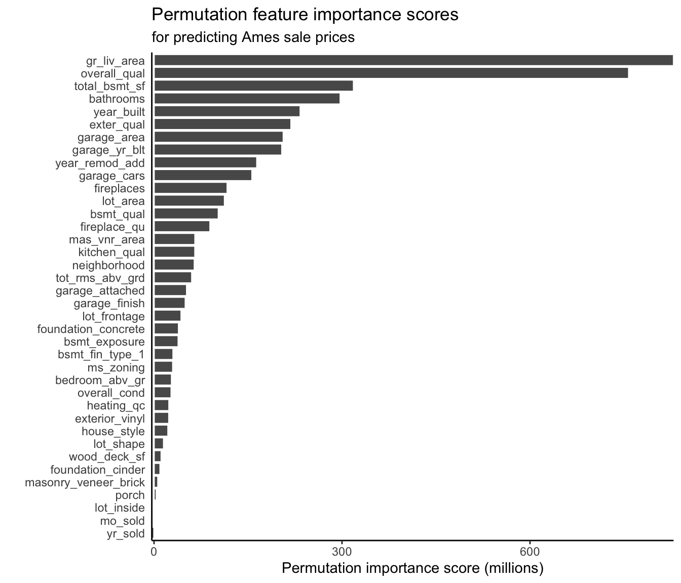
For the continuous response RF algorithm (with default hyperparameters) trained to predict house sale prices in Ames, Iowa, the permutation feature importance scores are shown in Figure 12.5. As with our LS coefficient-based findings, we again find that the most important features are the greater living area and the overall quality score.
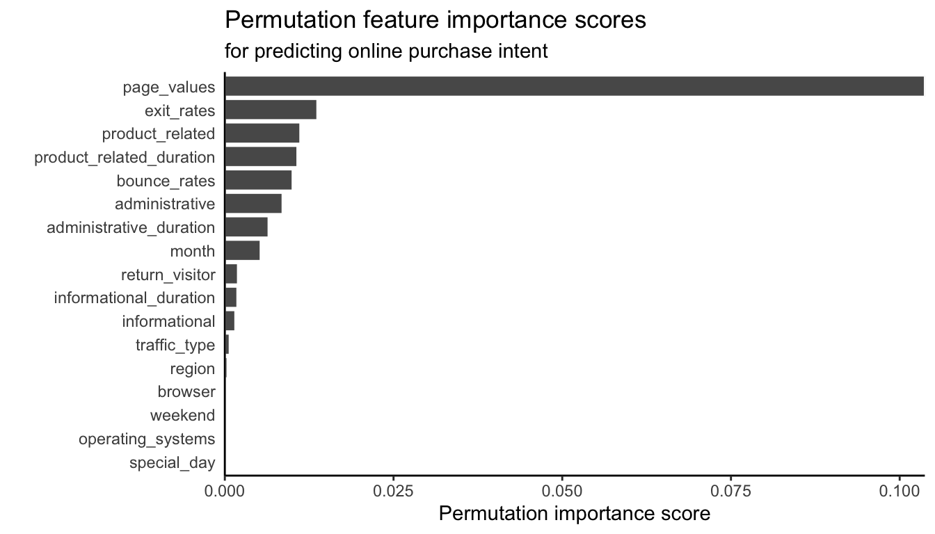
For the binary response RF algorithm (with default hyperparameters) trained to predict the purchase intent of online shopping sessions, the permutation feature importance scores are shown in Figure 12.6. It seems as though the page values feature is again the most important feature (matching what we found when looking at the standardized coefficients from the LS and logistic regression fits from Chapter 11).
12.4.2 The Gini Impurity Feature Importance Score
Another common feature importance score for the RF algorithm involves the Gini impurity for binary response problems and the corresponding variance measure for continuous response problems (i.e., the loss involved in choosing each split in the individual trees). Recall that the Gini impurity/variance of the child nodes will always be less than that of the parent node. It is also the case that the greater the reduction in impurity/variance from parent to child node, the better the split. Thus, the Gini impurity feature importance score for feature \(x\) can be computed by aggregating the decreases in Gini impurity (binary) or variance (continuous) across each split involving feature \(x\) across all the trees in the forest. This Gini impurity-based feature importance score is sometimes referred to as the mean decrease in impurity (MDI).
In the R ranger() implementation of the RF algorithm, the Gini impurity feature importance score can be computed by specifying the importance = "impurity" argument. In the Python implementation, the ensemble.RandomForestClassifier() class object provides a feature_importances attribute containing the impurity-based importance values.
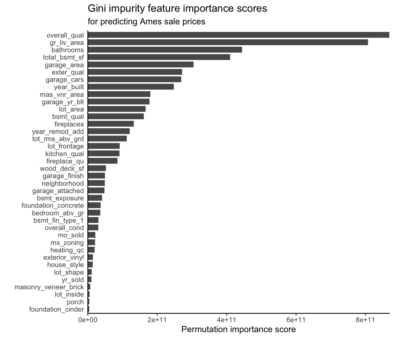
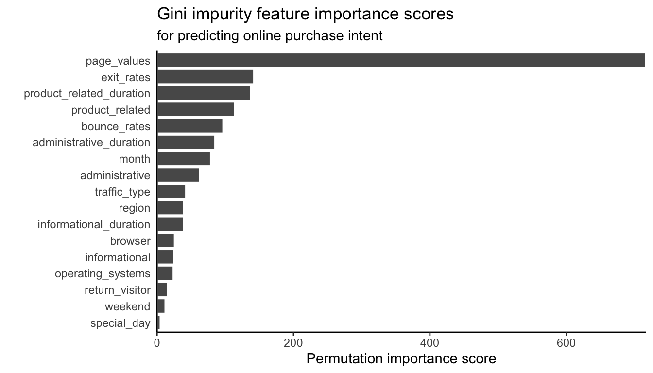
Figure 12.7 shows this variance-based Gini impurity feature importance measure for each predictive feature of the (continuous response) house sale prices, and Figure 12.8 shows the corresponding Gini impurity feature importance measure for each predictive feature of the (binary response) online purchase intent. Our findings are very similar to the permutation-based feature importance measures for RF, as well as the relevant LS and logistic regression variable coefficient-based importance evaluations.
Documentation and code for implementing and visualizing these feature importance scores for each project can be found in the 06_prediction_rf.qmd (or .ipynb) file in the relevant ames_houses/dslc_documentation/ subfolder for the ames housing project and the 04_prediction_rf.qmd (or .ipynb) file in the relevant online_shopping/dslc_documentation/ subfolder for the online shopping project, both of which can be found in the supplementary GitHub repository.
12.5 PCS Evaluation of the CART and RF Algorithms
Let’s compare the CART and RF algorithms to the LS (for continuous responses) and logistic regression (for binary responses) algorithms by conducting a predictability, computability, and stability (PCS) analysis of each algorithm. The code for the PCS analyses of the continuous response Ames house price prediction project can be found in the 06_prediction_rf.qmd (or .ipynb) file in the ames_houses/dslc_documentation/ subfolder, and the code for the PCS analysis of the binary response online shopping purchase prediction project can be found in the 04_prediction_rf.qmd (or .ipynb) file in the online_shopping/dslc_documentation/ subfolder, all of which are in the supplementary GitHub repository.
12.5.1 Predictability
As usual, the following predictability assessments are based on the predictive algorithms that have been trained using the “default” cleaned and preprocessed version of the training data for each project, and the evaluations are conducted on the corresponding validation set.
12.5.1.1 Ames Housing Sale Price Project (Continuous Response)
For the continuous response Ames house price prediction project, the validation set root-mean squared error (rMSE), mean absolute error (MAE), and correlation values for the RF algorithm (with default hyperparameters), as well as the CART and LS algorithms, each trained using the default cleaned/preprocessed version of the Ames training data and evaluated using the corresponding validation data, are displayed in Table 12.3. Notice that the RF algorithm performs better than the other two algorithms across all predictive performance measures.
| Fit | rMSE | MAE | Correlation |
|---|---|---|---|
| CART | 38,881 | 28,105 | 0.827 |
| LS | 23,267 | 17,332 | 0.942 |
| RF | 19,735 | 14,046 | 0.960 |
12.5.1.2 Online Shopping Purchase Intent Project (Binary Response)
For the binary response online shopping purchase intent project, we use the RF algorithm to compute purchase probability predictions and then convert these probabilities to a binary prediction using the 0.161 threshold value. Table 12.4 shows the validation set accuracy, true positive rate, true negative rate, and area under the curve (AUC) for the RF, CART, and logistic regression algorithms, each trained on the default version of the cleaned/preprocessed training dataset and evaluated using the corresponding validation set.
| Fit | Accuracy | True pos. rate | True neg. rate | AUC |
|---|---|---|---|---|
| CART | 0.886 | 0.818 | 0.897 | 0.874 |
| Logistic regression | 0.821 | 0.793 | 0.826 | 0.898 |
| RF | 0.846 | 0.876 | 0.840 | 0.935 |
Notice that for the specific threshold of 0.161, the RF algorithm does not achieve better accuracy or true negative rate than the CART algorithm. However, the RF algorithm achieves a higher true positive rate and AUC than the other algorithms, the latter of which indicates that the RF fit has greater predictive potential overall across a range of threshold choices. This is confirmed in Figure 12.9, which shows the validation set ROC curves for the RF, CART, and logistic regression purchase probability predictions.
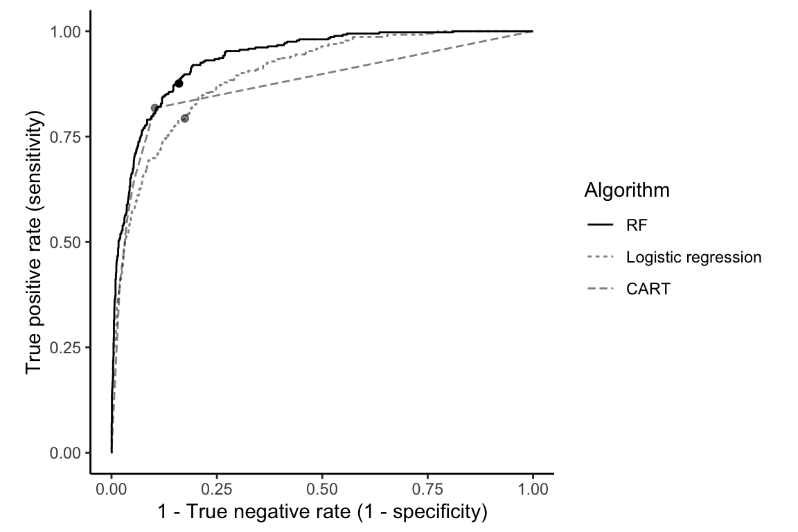
The fact that the RF ROC curve almost always sits above the other two ROC curves implies that there are threshold values for which the RF algorithm can always achieve a higher true positive rate for a given true negative rate (although the threshold may not have the same value for each algorithm).
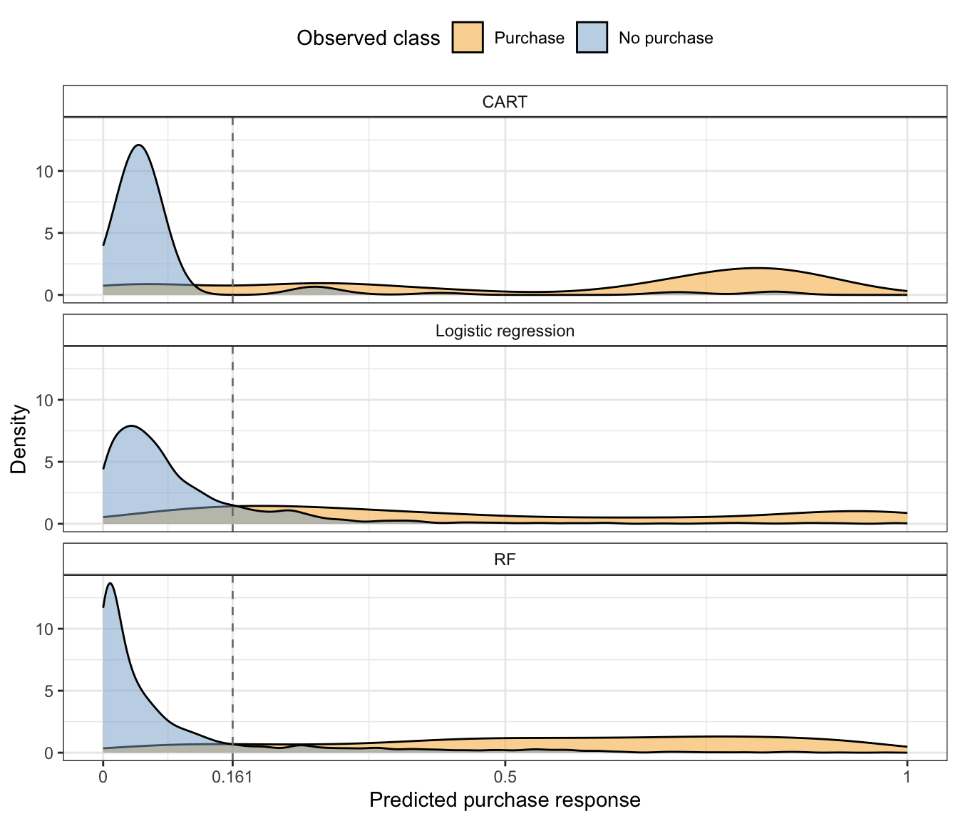
Finally, Figure 12.10 shows the distribution of the CART, logistic regression, and RF predicted purchase probabilities for the validation sessions for each class. For each algorithm, we see that there is a clear peak of low purchase probability values for the sessions that did not result in a purchase, and this peak is centered farther to the left for the RF algorithm relative to the CART and logistic regression algorithms (indicating that the RF algorithm is better at correctly detecting when a session is unlikely to end in a purchase). The predicted probabilities for the sessions that did end in a purchase are spread fairly evenly throughout the entire probability range for all three algorithms (indicating that none of them can easily detect when a session is likely to result in a purchase).
12.5.2 Stability
Next, let’s compare the stability of the LS/logistic regression, CART, and RF algorithms for each project.
12.5.2.1 Ames Housing Sale Price Project (Continuous Response)
Figure 12.11 shows a prediction stability plot for the range of predictions computed for 150 randomly sampled validation set Ames houses from each algorithm, each trained on 100 data– and 336 judgment call–perturbed versions of the training data (the relevant data and judgment call perturbations were described in Section 10.6.2.1 of Chapter 10).
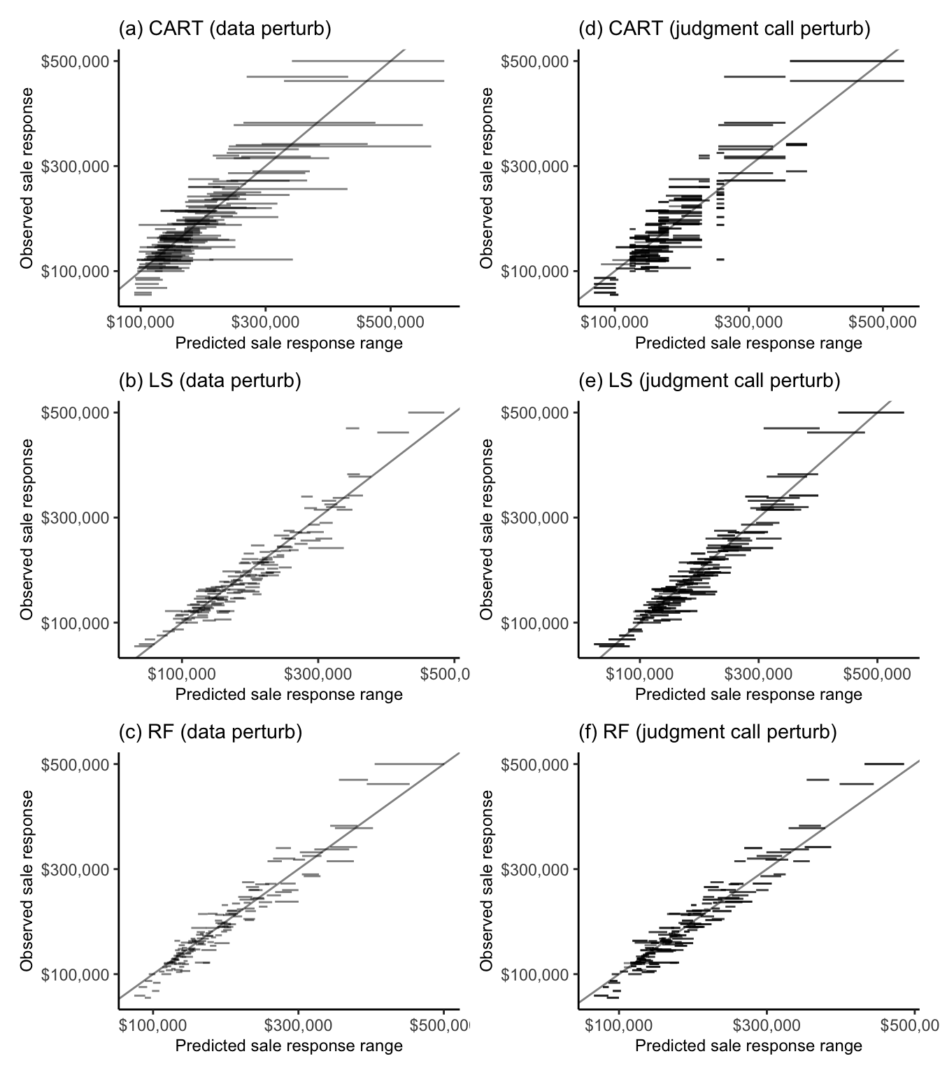
It is clear from Figure 12.11(c) and (f) that the RF algorithm is substantially more stable to both the data perturbations and cleaning and preprocessing judgment call perturbations than both the CART and LS algorithms. Indeed, the average standard deviation of the individual data-perturbed validation set sale price predictions from the RF algorithm is $3,970 (compared with $19,449 for the CART algorithm and $5,827 for the LS algorithm). Similarly, the average SD of the cleaning/preprocessing judgment call-perturbed RF sale price predictions for the validation set houses is $4,901 (compared with $11,875 for the CART algorithm and $9,330 for the LS algorithm).
It is worth noting that the prediction errors arising from the cleaning/preprocessing judgment call perturbations have a similar magnitude to those that arise from the bootstrap-based sampling data perturbations that we applied to our default cleaned/preprocessed training dataset. Recall, however, that in traditional statistical practice, only sampling-based data perturbations are used to evaluate uncertainty (traditional statistical practice does not consider judgment call perturbations). Our findings therefore imply that by ignoring the uncertainty arising from judgment calls, these traditional approaches to uncertainty assessment dramatically underestimate the overall uncertainty associated with data-driven results.
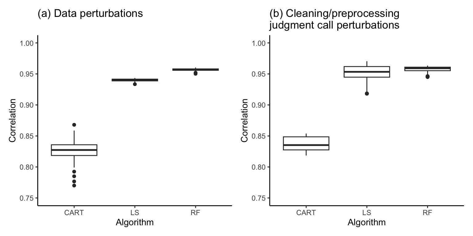
Figure 12.12 shows the distribution of the relevant validation set correlation performance measure for the continuous response Ames house price project fits for each algorithm trained on each of (a) the 100 different data–perturbed versions of the default cleaned/preprocessed Ames training dataset, and (b) the 336 different cleaning/preprocessing judgment call–perturbed versions of the training dataset. Overall, the RF algorithm correlation performance measure seems to be very stable relative to the other algorithms.
12.5.2.2 Online Shopping Purchase Intent Project (Binary Response)
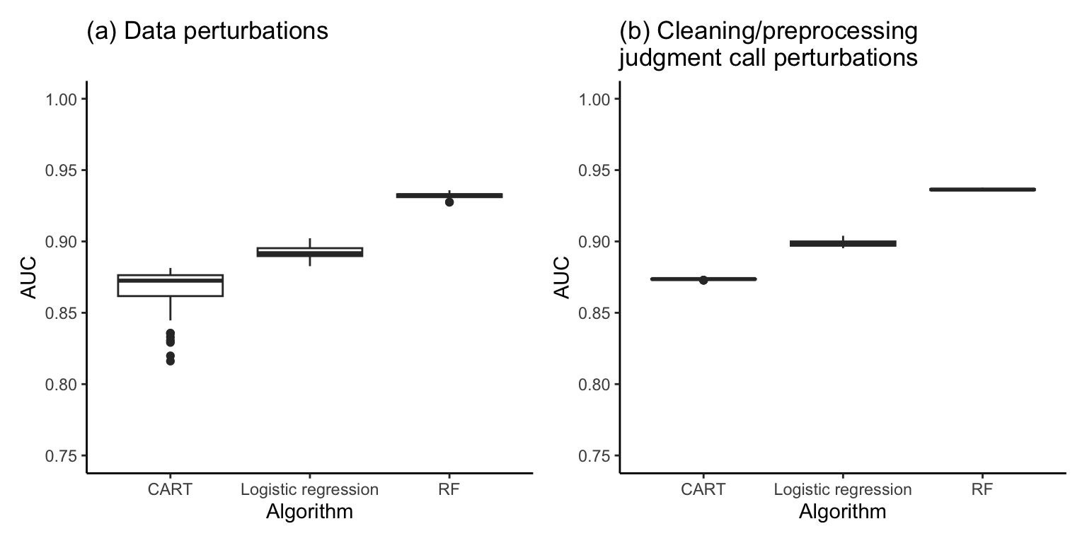
The data and cleaning/preprocessing judgment call perturbations that we will consider in this section are summarized in Section 11.5.2 of Chapter 11. Figure 12.13 shows the distribution of the validation set AUC across the (a) 100 data-perturbed and (b) the 16 cleaning/preprocessing–perturbed versions of each CART, logistic regression, and RF algorithm for predicting online shopping purchase intent. Notice that the AUC performance is very stable in each case (the widths of the boxplots are very narrow, indicating that the performance barely changes at all across the data and cleaning/preprocessing judgment call perturbations).
Exercises
True or False Exercises
For each question, specify whether the answer is true or false (briefly justify your answers).
You can compute predictions from a reasonably small decision tree without using a computer.
The CART algorithm can only be used to construct decision trees for predicting binary responses.
Even though the default CART hyperparameters typically lead to fairly good predictive performance, the predictive performance can often still be improved by tuning the hyperparameters.
The CART algorithm is always more stable to both data perturbations and cleaning/preprocessing judgment calls than the LS algorithm.
The Gini impurity measure can be used to evaluate the validation set predictive performance of the CART algorithm.
The CART algorithm is a random algorithm (meaning that it will result in a different fit every time you train it on the same data set).
The RF algorithm is a random algorithm (meaning that it will result in a different fit every time you train it on the same data set).
The Gini feature importance measure can only be used to compare the importance of predictive features that have been standardized.
The permutation importance measure is a general technique that can be used for algorithms other than the RF algorithm.
Applying a log-transformation to a predictive feature does not affect the prediction output of the CART algorithm.
Conceptual Exercises
The continuous response CART algorithm chooses each split by minimizing the loss function defined by the variance of the responses in the resulting child nodes. Provide an alternative loss function that you might use to choose each split for a decision tree with continuous responses (you don’t have to implement your idea, and you don’t need to provide a formula; you can just describe what quantity your proposed loss function would measure).
Describe the two ways in which the RF algorithm introduces randomness into each individual tree, and discuss at least one alternative technique you could use to introduce additional randomness into the RF algorithm.
Explain how you could apply regularization to the RF algorithm and why you might want to regularize it.
Mathematical Exercises
Compute the Gini impurity for the following potential splits of a set of 30 observations (8 of which are in the positive class and 22 of which are in the negative class).
Split option 1: The left child node has 7 positive class observations and 10 negative class observations, and the right child node has 1 positive class observation and 12 negative class observations.
Split option 2: The left child node has 8 positive class observations and 8 negative class observations, and the right child node has 0 positive class observations and 14 negative class observations.
Split option 3: The left child node has 7 positive class observations and 3 negative class observations, and the right child node has 1 positive class observation and 19 negative class observations.
Based on the Gini impurity for each of the splits listed in the previous steps, which split would you choose?
Coding Exercises
Conduct a data perturbation stability evaluation of the RF feature importance analysis for both the continuous response Ames house price project and the binary response online shopping project. You may want to conduct your analysis in the relevant files from the supplementary GitHub repository (i.e., in the
06_prediction_rf.qmdor.ipynbfile in theames_houses/dslc_documentation/subfolder for the Ames house price project and the04_prediction_rf.qmdor.ipynbfile in theonline_shopping/dslc_documentation/subfolder for the online shopping project).For both the continuous response Ames house price project and the binary response online shopping project, write a function in R or Python that computes to a simplified version of the RF algorithm that consists of an ensemble of three CART algorithms (e.g., each trained using the
rpart()CART function in R or thetree.DecisionTreeClassifier()class from the scikit-learn Python library). Each of the three CART algorithms that make up the ensemble should be trained on a bootstrapped version of the default cleaned and preprocessed training dataset (but you do not need to implement the random feature selection for each split).Using the continuous response Ames house price data, demonstrate that the predictions generated by the CART algorithm are not affected by monotonic transformations (e.g., logarithmic or square-root transformations) of the predictor variables. Hint: one way to do this is to compute two different CART fits, one in which one or more of the predictor variables have been transformed, and another in which they have not, and compare the predictions produced by each fit.
Use CV to train the RF hyperparameters corresponding to the number of variables to try at each split (
mtryin the “ranger” implementation in R andmax_featuresin the scikit-learnensemble.RandomForestClassifier()class in Python) and the minimum number of observations required to split a node (min_nin the “ranger” implementation in R andmin_samples_splitforensemble.RandomForestClassifier()in Python) for both the continuous response Ames house price project and for the binary response online shopping project. You can use the default values for all other hyperparameters. Here, we provide a suggested procedure for how to do this (although you may choose to do it differently):Start by choosing three or four plausible values for the hyperparameter.
Split the training dataset for each project into \(V=10\) equally sized, nonoverlapping subsets (folds).
Iterate through each hyperparameter value, and conduct a CV evaluation for each value. We recommend using the AUC as your performance measure.
For each hyperparameter value, compute the average CV AUC for the withheld folds.
Identify whether there is a clear choice of hyperparameter value that yields the “best” CV AUC performance. You may want to print a table and/or create a visualization to do this.
Train an RF algorithm using the CV-tuned hyperparameter value and compare the validation set predictive performance with an RF that is trained using the default hyperparameter values.
Project Exercises
Predicting house affordability in Ames Repeat the housing affordability binarization project exercise from exercise 26 in Chapter 11, this time using the RF algorithm with the perturbation and impurity importance features. Compare your results from the LS and logistic regression fits from exercise 26 in Chapter 11.
Predicting happiness (continued) This project extends the continuous response happiness prediction project from the project exercises in Chapter 9 and Chapter 10 based on the World Happiness Report data. The files for this project can be found in the
exercises/happiness/folder on the supplementary GitHub repository.In the
03_prediction.qmd(or.ipynb) code/documentation file in the relevantexercises/happiness/dslc_documentation/subfolder, use the CART and RF algorithm to compute two predictive fits for the happiness score.Conduct a PCS analysis of your CART and RF fits, and compare your fits to those you created for the Chapter 10 project exercise.
Compute the perturbation and impurity importance scores to identify which variables are most important for predicting happiness. How does it compare to your coefficient-based findings from the project in Chapter 10?
Predicting patients at risk of diabetes (continued) This project extends the binary response diabetes risk prediction project from Chapter 11, based on the data from the 2016 release of the National Health and Nutrition Examination Survey (NHANES). The files for this project can be found in the
exercises/diabetes_nhanes/folder on the supplementary GitHub repository.Continuing to work in the same
03_prediction.qmd(or.ipynb) file in theexercises/diabetes_nhanes/dslc_documentation/subfolder that you used for the Chapter 11 project, train predictive fits of diabetes status using the CART and RF algorithms.Conduct a thorough PCS analysis of each of your fits and compare with your LS and logistic regression fits that you fit in the diabetes project exercise from Chapter 11. Your PCS analysis should involve evaluating your predictions on the validation set and investigating the stability of your predictions to reasonable data perturbations and cleaning and preprocessing judgment calls.
References
Breiman, Leo. 2001. “Random Forests.” Machine Learning 45 (1): 5–32.
Breiman, Leo, Jerome H. Friedman, Richard A. Olshen, and Charles J. Stone. 1984. Classification and Regression Trees. Chapman; Hall/CRC.
Goodfellow, Ian, Yoshua Bengio, and Aaron Courville. 2016. Deep Learning. MIT Press.
Hastie, Trevor, Jerome Friedman, and Robert Tibshirani. 2001. The Elements of Statistical Learning. Springer. Springer.
Wright, Marvin N., and Andreas Ziegler. 2017. “Ranger: A Fast Implementation of Random Forests for High Dimensional Data in C++ and R.” Journal of Statistical Software 77 (March): 1–17.
Each of these algorithms can be thought of as a sophisticated extension of the LS and logistic regression algorithms that we have already introduced.↩︎
While the R implementations of these algorithms accept categorical variables, the Python scikit-learn implementations still require that they first be converted to numeric variables.↩︎
Although LS can technically be used to predict binary responses, it was not designed to do so.↩︎
This is true when there are only two classes, but it may not be the case for multiclass problems (although we don’t consider multiclass problems in this book).↩︎
To compute probability predictions while using the
ranger()implementation of the RF algorithm in R, use the argumentprobability = TRUE.↩︎The specific names of these hyperparameters vary across software implementations.↩︎