1 An Introduction to Veridical Data Science
This is a pre-release of the Open Access web version of Veridical Data Science. A print version of this book will be published by MIT Press in late 2024. This work and associated materials are subject to a Creative Commons CC-BY-NC-ND license.
To practice veridical data science is to practice “truthful” data science. The goal of veridical data science is to answer real-world questions by collecting and critically evaluating relevant empirical (data-driven) evidence using human judgment calls in the context of domain knowledge. If the empirical evidence is deemed sufficiently trustworthy, it is communicated to domain stakeholders, where it can play a role in real-world decision making and updating domain knowledge.
The overall goal of most data science projects is to use the insights gained from data analyses to help us make decisions in the real world. For instance, demographers conduct and analyze surveys on members of a human population of interest to help guide policy decisions, ecologists observe and analyze data on animal and plant distributions and behaviors to help make conservation decisions, and financial analysts evaluate financial market trends to help make financial decisions.
1.1 The Role of Data and Algorithms in Real-World Decision Making
Obtaining data-driven insights typically involves implementing algorithms that are designed to summarize and extract the relevant patterns and relationships that are hidden within a dataset. An algorithm is a set of instructions that tell your computer how to perform a specific task (such as summarizing a particular pattern). Since humans chose the set of instructions that define each algorithm, each algorithm is a mental construct that is intended to represent certain types of relationships that we hypothesize to be meaningful in our data. We use the term “algorithm” fairly broadly. For example, in addition to “machine learning (ML) algorithms”, which generate predictions of a response, you could think of computationally calculating the mean as an algorithm that adds up a collection of numbers and then divides by the number of numbers in the collection. You could even think of the process of creating a scatterplot as a data visualization algorithm that takes a collection of pairs of numbers and arranges them as points in two dimensions.
The relevance of an algorithm to the real world is upper-bounded by the extent to which the data that underlies it reflects reality. Unfortunately, data almost never perfectly captures the real world that it was designed to measure. A poorly thought-out or poorly followed data collection protocol may result in a dataset that does not adequately represent the intended real-world population, and imprecise instruments and human approximations can lead to incorrect values being entered into a dataset. Unless we know with certainty what the “true” values of each of the real-world quantities being measured are (which we generally don’t, since we only see our own measurements of these quantities), we typically don’t know how accurate the values in any given dataset are. Moreover, even if our original data is a reasonable reflection of reality, when we clean and preprocess our data so that we can conduct computations with it, we modify it. While these modifications are typically intended to bring our data more in line with reality, they are based on our own judgment calls and assumptions about the real-world quantities that the measurements in our data are supposed to represent. However, mistaken assumptions may unintentionally diminish the relationship between our data and reality.
However, these issues are not only relevant for the current data that we use to conduct our analyses and fit our algorithms, they are also true for the future data to which we will apply them. For instance, although a demographer might have analyzed a survey that involved 500 Americans, the end goal is to use this information to help understand and make future decisions for all Americans (in this case, the current data corresponds to the 500 Americans involved in the survey on the date when the survey was taken, and the future data corresponds to all Americans in a time period following the survey). Similarly, a financial analyst might train an algorithm for predicting financial market trends based on data from the past 10 years, but their goal is to apply their algorithm to predict and understand future market trends. In each case, the future data being used to make real-world decisions is similar to—but certainly not the same as—the current data used to conduct the analysis and fit the algorithms.
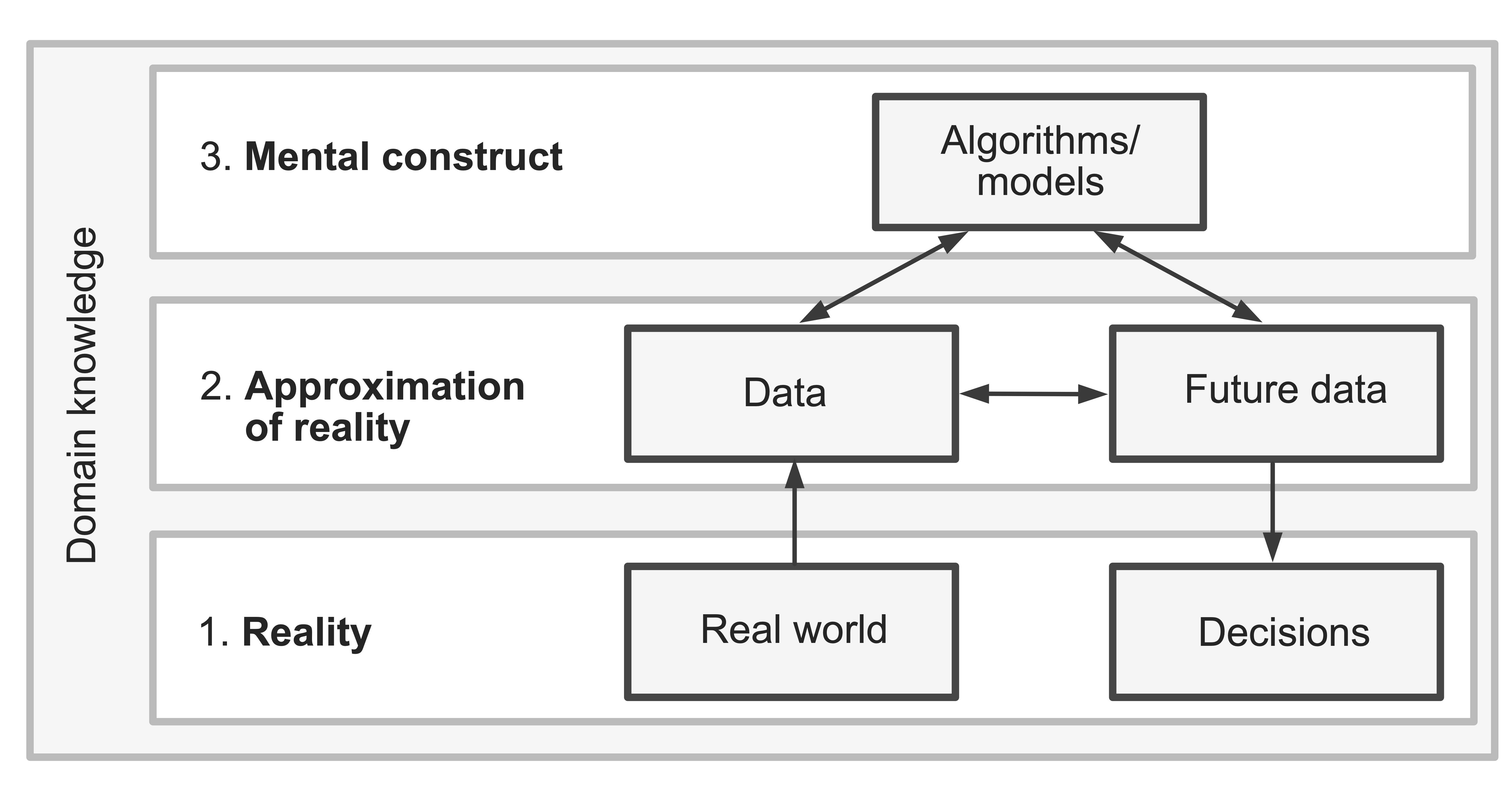
If we want the real-world decisions that we make based on our algorithms to be trustworthy, we thus need the current data that underlies our algorithms and the future data to which we want to apply them to reasonably reflect reality and to be similar to one another.1 We also need the algorithms that we fit to be able to reliably capture the patterns and relationships that are contained within both the current and future data. That is, we need strong connections between the three realms (Figure 1.1), which are (1) the real-world realm (where we live); (2) the data realm (which is an approximation to reality and is where our data lives); and (3) the algorithmic realm (where the algorithms that are mental constructs designed to represent our data live).
The problem is that we usually don’t know how strong the connections among these three realms are, and making real-world decisions based on results from algorithms that don’t represent reality (whether due to the data being a poor approximation of reality or the improper use of analytic techniques) can lead to untrustworthy results that can have drastic real-world consequences. Consider the example of facial recognition software. It has been well-documented that many software applications designed to recognize faces using images are much better at recognizing the faces of light-skinned people than dark-skinned people. One of the primary drivers of this issue is that these algorithms were built primarily using images from people with light skin (i.e., the data did not reflect the diversity that exists in the real world) (Khalil et al. 2020). When biased data is used to train facial recognition software, the resulting software will typically also be biased, and when used in the real world, these biases can lead to the exacerbation of existing societal inequalities.
Since your data will not inform you whether it is accurately representing reality, nor will your algorithms warn you when they are being used inappropriately, you need to conduct some data-detective (critical thinking) work to determine whether your data is a reasonable reflection of reality and whether your algorithms are being applied appropriately to your data and domain problem. In Section 1.2, we will introduce some critical thinking questions that you can ask that will help you use relevant domain knowledge to assess the trustworthiness of data-driven results qualitatively in terms of how accurately the data reflects reality and how appropriate the analyses and algorithms are in the context of the data and domain problem. Then, in Section 1.3, we will introduce the principles of predictability, computability, and stability (PCS), which we will use throughout this book to assess the trustworthiness of data-driven results quantitatively in terms of how applicable the results are to relevant future data scenarios and how sensitive they are to reasonable perturbations in our data and analysis pipeline (including the human judgment calls that we make when cleaning, preprocessing, and analyzing data).
1.2 Evaluating and Building Trustworthiness Using Critical Thinking
Data science involves more than just doing math and writing code; it also requires strong critical thinking skills and a foundation of domain knowledge relevant to the project that you’re working on (which can be obtained from your own expertise, the internet, books, or your collaborators). These skills are crucial for identifying potential weaknesses in the connections between the three realms, described above, and for detecting biases that might sneak into the data collection and analysis pipeline. Without strong critical thinking skills and basic domain knowledge (even if just from a literature review), you run the risk of producing misleading results that can have dire real-world consequences.
Unfortunately, statistics and data analyses have a poor reputation for trustworthiness among the general public, with sayings such as “There are three kinds of lies: lies, damned lies, and statistics2” commonly interrupting casual discussions about data analysis. As much as we would love to say that this reputation is undeserved, we can’t deny that it is very easy to use data to lie. The problem is that most of the time, these lies are unintentional, resulting from a lack of critical thinking and a failure to thoroughly scrutinize data-driven results (e.g., using the principles of PCS that we will introduce below) before presenting them as “facts.”
A data scientist who is well versed in critical thinking and domain knowledge (and/or is working closely with domain experts), who possesses a reasonable understanding of the algorithms being used (including the relevant assumptions and pitfalls), and who embraces the principles of PCS, is substantially less likely to fall into the trap of unintentionally lying with data. Next time you hear someone say, “There are three kinds of lies: lies, damned lies, and statistics,” rather than getting offended, you can instead correct them: “There are three kinds of lies: lies, damned lies, and bad statistics.” Not all data science projects involve bad data analysis, but some certainly do!
Some critical thinking techniques that we recommend employing throughout every data science project (and to assess other people’s projects) include the following:
Asking questions about the domain problem. Is the question being framed really the question you care about, and is this question ethical in the first place? For example, if you have been presented with the business question “Which features of our website can we change that will make our customers less likely to cancel their subscription?” you might find that one answer is to move the “Cancel subscription” button to a more discrete (i.e., harder-to-find) location. But is this really the question that you want to ask? Is it ethical? A better question might have been, “Why do customers tend to cancel our product subscription?” The answer to that question could help your company improve your product offerings (rather than just make it harder for your customers to cancel).
Asking questions about the data. Where did the data come from? Is the source of the data trustworthy? Is the data relevant to the question being asked, as well as any future setting to which the results might be applied? What do the values contained within the data actually correspond to in the real world? These questions are a great way to catch inconsistencies and errors that might otherwise derail your analysis. Try to imagine yourself being physically present during data collection. What potential issues might arise? Whenever possible, do the “shoe-leather” work (Freedman 1991).
Asking questions about the analysis, algorithms, and results. What do these results mean in the context of reality? Do they make sense? Do the analysis and algorithms involve making any assumptions about the data or domain? Are these assumptions reasonable? Do these results answer the primary project question? Are the results being communicated accurately?
In addition to these questions, it is important to keep an eye out for confirmation bias and desirability bias. Confirmation bias occurs when you fail to critically scrutinize results because they match what you expect to find. As human beings, we’re a lot more likely to double-check and scrutinize our results when they don’t match our expectations (which means that we’re a lot less likely to catch errors when the results match what we expect). Desirability bias occurs when you try to find the results that you think other people (or popular opinion) expect you to find.
What can you do to diminish the risks of confirmation and desirability bias? While it’s impossible to let go of your expectations entirely, you can work on developing a healthy skepticism of every result that you obtain, regardless of whether it matches what you or other people expected or wanted to find.
1.2.1 Case Study: Estimating Animal Deaths Caused by the 2019 Australian Bushfires
Let’s use our critical thinking skills to do some detective work using an example that comes from the horrific bushfires that ravaged over 42 million acres of the east coast of Australia for many months during late 2019 and into 2020 (to put this in perspective, this is an area larger than the entire state of Florida). A number of scientists (the most prominent of whom was Professor Chris Dickman at the University of Sydney, who has over 30 years of experience working on the ecology, conservation, and management of Australian mammals) estimated that “over 1 billion animals perished in the fires.” That number, 1 billion, is absolutely staggering. While most people will accept reports of scientific studies without question, we are not most people. Let’s spend some time thinking critically about where this mind-boggling number, 1 billion, might have come from (not to downplay the undeniably horrific consequences of these fires, but rather, to better understand them).
1.2.1.1 Asking Questions about the Data
How do you think the data that underlies the statement that “1 billion animals perished in the fires” was collected? Was there a team of scientists manually counting every single animal that died? Does the term “animal” include insects, such as ants and flies? Fortunately, with a little bit of research, we were able to find answers to these questions fairly quickly. We encourage you to try to answer any questions of your own too. A quick internet search led us to a news article (University of Sydney 2020), stating that Professor Dickman based his estimations on a detailed study by Johnson et al. (2007) (13 years before the fires happened) on which Professor Dickman was a coauthor:
“The figures quoted by Professor Dickman are based on a 2007 report for the World Wide Fund for Nature (WWF) on the impacts of land clearing on Australian wildlife in New South Wales... [which contained] estimates of mammal, bird and reptile population density in NSW” (University of Sydney 2020).
PDF copies of both of these articles (Johnson et al. 2007) and (University of Sydney 2020) are provided in the bushfires/ folder of the supplementary GitHub repository for the interested reader.
What we found in our literature search is that these estimates were based on data collected in 2007, and further reading revealed that this study only covered a small region of the state of New South Wales. The report from University of Sydney (2020) also stated that “the figure includes mammals (excluding bats), birds and reptiles and does not include frogs, insects or other invertebrates.”
From this information, we can conclude that these results were not based on some mystical database that contained information on all the animals that died in the fires, likely because no such data exists (and trying to imagine collecting such a dataset quickly leads us to conclude that it would be an impossible task). Although the data that underlies the results come from a verifiable and legitimate source (the 2007 study conducted by the World Wildlife Fund, a reputable organization), this doesn’t automatically mean that it is relevant to the question being asked. A lot can change in 13 years, and it is a big claim to say that the estimates collected from a small, localized habitat can be generalized to the entire region affected by the fires.
The data that underlie this study is thus relevant, but there is no doubt that it is limited in scope. At the end of the day, Professor Dickman did his best with an existing dataset that he was already familiar with, given that there was no other relevant data available. Often, the best data is just the data you have.
1.2.1.2 Asking Questions about the Analysis
Given that the data was based only on a small, localized region, how did Professor Dickman and his collaborators use the data to approximate the number of animals that died across the entire affected region? From the University of Sydney (2020) report, we learn that
“Estimates of mammal, bird, and reptile population density in NSW [were obtained by multiplying] the density estimates by the areas of vegetation approved to be cleared” (University of Sydney 2020).
We interpret this to mean that they took the 2007 estimates of animal densities and scaled up these numbers based on the size of the affected area. This approach obviously does not take into account differences in animal densities across the entire affected area, nor does it take into account how these densities may have changed over time. However, given that no additional data was available, what else could they do?
While we can criticize other people’s data-driven conclusions all we want, in many cases they are the best (and often the only) figures available. When criticizing someone else’s study, always keep in mind that behind every data-driven conclusion is a well-intentioned human being with feelings (something that people often conveniently forget). In the case of Professor Dickman’s study, while perhaps we shouldn’t take the claims as a base truth (the authors themselves were very clear in their report that these are rough estimates and should not be taken literally), they do paint an impactful picture of the devastating consequences of the fires on the local animal populations given the information available. Moreover, this was the first high-profile study that even attempted to quantify the impact of the fires on the animal populations.3
By thinking critically about the numbers reported concerning the impact of these fires, we can gain a much clearer understanding of where they came from and how we should interpret them. In your own studies, our advice is to always be transparent about the assumptions that underlie your data and results and document them (publicly, if possible). Every data-driven result has caveats, and it is your job to ensure that your results are being interpreted as accurately as possible.
1.3 Evaluating and Building Trustworthiness Using the PCS Framework
While these critical thinking questions help provide a general qualitative measure of the trustworthiness of data-driven results, it is often important to also provide quantitative measures. This is where the predictability, computability, and stability (PCS) principles come in. These principles were first introduced in Yu and Kumbier (2020), but have been greatly expanded in this book.
The PCS framework offers guidance and techniques for empirically demonstrating that your results hold up to some predictability reality checks and stability evaluations that address various sources of uncertainty associated with your result. The three PCS principles are:
Predictability. Your conclusions are considered to be predictable if you can show that they reemerge in relevant future data and/or are in line with existing domain knowledge. Predictability evaluations can be thought of as a reality check. We will expand on the predictability principle in Section 1.3.1.
Computability. Computability is the workhorse behind every data analysis, PCS evaluation, and simulation study. You typically don’t need to demonstrate that your results are computable; rather you will use computation to conduct and evaluate your analyses, as well as to create data-inspired simulations.
Stability. Your conclusions are considered stable if you can show that they remain fairly consistent when realistic perturbations (changes/modifications) are made to the underlying data, judgment calls, and algorithmic choices. Stability assessments can be thought of as a set of stress-test evaluations of the uncertainty that is associated with your data-driven results. We will expand on the stability principle in Section 1.3.2.4
Predictability and stability assessments are a powerful means of providing evidence for the trustworthiness of your data-driven results. They do not, however, allow you to prove that your data-driven results are trustworthy. Absolute proof would require completely exhaustive predictability and stability assessments that consider all possible alternative data and analytic scenarios—an impossible task. These ideas contain echoes of “Popperian falsification,” as defined by the philosopher Karl Popper in the 1930s (Popper 2002). Popperian falsification5 states that a scientific finding is never really proven, but rather, every positive experimental result demonstrates further evidence for the scientific finding.
While the PCS framework itself is new, many of the ideas that underlie it are not. The PCS framework aims to unify, streamline, and expand on the existing best practices and ideas from ML, statistics, and science.
1.3.1 Predictability
Scientists have been conducting predictability reality checks for centuries. For instance, in the early 1800s, Carl Friedrich Gauss developed a model for predicting the location of the asteroid Ceres in the sky, and he checked his model (i.e., he showed that it generated predictable results) by demonstrating that it accurately predicted Ceres’s actual future location. In a more modern setting, the ML community has long been demonstrating predictability by evaluating their algorithm’s performance on withheld validation and test sets. The PCS framework’s predictability principle expands the role of domain knowledge and the use of a validation set broadly, beyond just prediction problems.
The most powerful predictability evaluation technique, however, involves demonstrating that your results reemerge in the context of the actual external or future data to which you will be applying them. For instance, if you have developed an algorithm for predicting stock prices (based on past stock market data) and you want to use your algorithm to predict future stock prices, you should show that your algorithm generates accurate predictions for stock market data that spans a time period that takes place after that of the data original used to “train” your algorithm. As another example, imagine that you are conducting an analysis to try and understand hospital-acquired infection risk factors using data collected from patients in the hospital where you work. If you intend to apply your findings to patients from other hospitals, then you should demonstrate that the risk factors that you identified are relevant to patients in other hospitals too.
However, there are many situations where you don’t have access to any external or future data that reflects the scenario in which you intend to apply your results or algorithms. In these situations, you can emulate future or external data by withholding some of your original data before conducting your analysis for the sole purpose of evaluating the predictability of your results. This withheld data can serve as a surrogate for future data (see Section 1.3.1.1). Additional evidence of the predictability of your results can be obtained from demonstrating that your analyses and algorithms are capable of capturing results and relationships that are well known in the domain field (see Section 1.3.1.2).
1.3.1.1 The Training, Validation, and Test Datasets
In the absence of available future/external data, the recommended technique for generating surrogate external/future datasets is to split your data into a training set and a validation set (and possibly also a test set), as is common in the ML community.
The training set (training data/training dataset) is the biggest portion of the data (which should contain at least 50 percent of the original data; we often use 60 percent), and this is the data that you will use to conduct your explorations, analyses, and to train your algorithms.
The purpose of the validation set (validation data/validation dataset) (we typically use 20 percent to 40 percent of the original data, depending on whether we are also creating a test dataset) is to provide an independent assessment of your results or algorithms: that is, to demonstrate that your results reemerge (or your algorithms perform well) in data that resembles the future data to which your results will be applied. The validation dataset should thus be created in such a way that best reflects actual external or future data on which your results might be used to conduct real-world decision making. Often, the validation dataset results will be used to decide between several alternative analyses or algorithms or to filter out poorly performing algorithms (this is particularly common in prediction problems). In that case, since your validation dataset has then been used to produce your final results, it becomes important to use another withheld dataset to provide an independent evaluation of your final results.
This is where the test set (test data/test dataset) comes in. The test set will consist of the remaining data that has not been used in the training or validation datasets, which is typically 20 percent of the original data. The test dataset can be used to provide a final independent assessment of an algorithm that was chosen based on the validation set performance. Similar to the validation dataset, the test dataset should resemble the future data to which your results will be applied as closely as possible.
If you will be using validation (and test) sets to evaluate your data-driven results, it is important that you set aside these subsets of your data before you start conducting your analyses.
If you are splitting your data into training, validation, and test datasets, you should do so in such a way that the validation and test datasets reflect the future/external data to which you intend to apply your results. Common splitting mechanisms include the following:
Time-based split: If your data was collected over time and you will be applying an algorithm that you have trained to future data, then a train/validation/test split that uses the earliest 60 percent of your original data as the training dataset, and evenly splits the later 40 percent of your data between the validation and test sets is a good representation of the relationship between the current and future data. For example, if you have 10 years of stock market data, you could use the stock prices from the first 6 years as your training data and then use stock prices from the final 4 years for the validation and test datasets for evaluation. In practice, however, after you have conducted your evaluations, you may want to re-train your algorithm using all of the available data to ensure that your algorithm is capturing the most up-to-date trends possible.
Group-based split: If your data has a natural grouping (e.g., if your data consists of information from patients from several different hospitals), and you will be applying an algorithm that you train to a new group of data points (e.g., to patients in a different hospital), then you might want to choose a random subset of 60 percent of the groups (e.g., hospitals, rather than patients) to form the training dataset, and then evenly split the remaining groups (e.g., hospitals) between the validation and test datasets. This ensures that every data point from the same group will be contained entirely within the training dataset, the validation dataset, or the test dataset, rather than split across them, and best reflects the process of applying the algorithm to data points in a new group (e.g., patients in a new hospital).
Random split: Using a purely random split to form the validation and test datasets (i.e., randomly selecting two sets of 20 percent of the data points to form the validation and test datasets) is reasonable when the current data points are all more or less exchangeable with one another (e.g., when people are randomly included in a survey), and the new data points to which you will be applying your results are similar to the current data points (e.g., you will be generalizing your results to other people who were not included in the survey, but could have been).
Regardless of the type of split you choose, you should always justify why your choice provides a good surrogate for the relevant future (or external) data using domain knowledge, your understanding of the data collection process, and how your results or algorithms will be used (e.g., what kind of future data they will be applied to).
Note that there is no specific need to feel tied to the 60/40 train/validation split (or 60/20/20 train/validation/test split): you can choose whichever proportions you feel comfortable with, although we recommend creating a training dataset that contains at least 50 percent of your data.
As a reminder, it is strongly recommended that you split your data into training, validation, and test datasets before you start exploring and analyzing your data (although it is all right to do some light explorations before splitting your data to get a sense of the data structure). Splitting your data in the very early stages of your project will help prevent data leakage, where information from your training dataset “leaks” into your validation and test sets (and vice versa), impairing the ability of the validation and test sets to meaningfully act as a reasonable surrogate of truly independent future or external data (Kaufman et al. 2012).
It is thus important to make a plan for how you will evaluate the predictability of your results very early in your project (ideally as soon as you have collected your data).
1.3.1.2 The Role of Domain Evidence in Demonstrating Predictability
While we will primarily use external/validation data to evaluate the predictability of our results, another technique that we will sometimes use to demonstrate the predictability of our results is to show that our analysis or algorithm uncovers well-established patterns or relationships in the domain field (e.g., from reputable peer-reviewed research articles).
For instance, if we develop an algorithm for identifying associations between genotypes (genes) and phenotypes (physical traits), and we can show that our algorithm is able to uncover known genotype-phenotype relationships (e.g., our results show that a gene well-documented in the literature to be associated with having red hair is indeed associated with the red hair phenotype), then we can use this as evidence of the predictability of our algorithm, which in turn provides evidence of the trustworthiness of any new relationships that we identify. This is an example of using the principle of predictability as a reality check.
1.3.2 Stability
The second pillar of the PCS framework is stability. To understand the principle of stability, consider the following metaphor. For every photograph that you take, there are multiple plausible alternative photographs that you could have taken, but didn’t. For example, the photograph could have been taken 30 seconds later, or you could have been standing three paces to the left. The same is true of the data that we collect. For every dataset that we collect, there are many plausible alternative datasets that we could have collected, such as if someone else had recorded the measurements, if they had been measured on a different day, or if the measurements had been taken for a slightly different set of individuals.
Our metaphor doesn’t stop at the stage of data collection though. After we take our photograph, there are many preprocessing filters that we can use to modify it, often with the goal of making the photograph look more like the real world that we see with our eyes. The processing choices that we make here are judgment calls. Therefore, for any given photo that we take, there are many alternative final products that we could plausibly end up with, resulting from taking a slightly different picture and/or using slightly different preprocessing techniques.
The analogy in data science is that there are many alternative ways that we can choose to clean or preprocess our data (e.g., there are multiple ways to impute missing values) as well as analyze it (e.g., there may be multiple algorithms that perform the same task), resulting in a wide range of possible downstream results that we can obtain. The uncertainty that underlies the data collection procedure and the cleaning and analysis judgment calls that we make manifest as uncertainty in our results.
For most data science projects, there is no single “correct” dataset to collect, nor is there a single “correct” way to clean or analyze it. Instead, there are many equivalent datasets that you could collect, many alternative data cleaning mechanisms that you could implement, and multiple analyses that you can conduct, each of which is equally justifiable using relevant domain knowledge. The question is: Across the spectrum of reasonable datasets, cleaning procedures, and analyses that we could have conducted, how variable are the alternative results that we could have obtained? If the answer is “very variable,” then our results are clearly very sensitive to the minute choices that were made during the process of generating them, and the question becomes: Should we trust that the particular set of results that we generated accurately reflect reality? We can find an approximate answer to this question by conducting a stability analysis.6
Like the predictability principle, the ideas that underlie the stability principle have a long history. Stability is an expansion of the concept of uncertainty assessment from classical statistics (as well as stability in numerical analysis and control theory). Uncertainty, in this context, refers to the ways in which our results might have looked different under various scenarios.
The classical statistical view of uncertainty considers just one source of uncertainty based on asking how the results might look different had an alternative random sample been collected; that is, it only considers sample variability under a hypothetical data collection/sampling process. The veridical data science stability principle, however, considers a much broader range of sources of uncertainty, asking how the results might look different had alternative data been collected (in ways beyond alternative random samples), as well as if we had made alternative cleaning, preprocessing, and analysis judgment calls. The stability principle can thus be thought of as an expansion of the traditional concepts of statistical uncertainty, as well as statistical robustness, which focuses on finding statistical parameter estimators that are stable across a wide range of statistical data collection mechanisms and distributions.
In this book, we primarily address three sources of uncertainty arising from three sources: (1) the data collection process using appropriate data perturbations; (2) the data cleaning and preprocessing judgment calls; and (3) the choice of algorithm used. If your results fall apart when you make alternative judgment calls at any of these stages, it indicates that they are unstable. The three uncertainty assessments that we focus on in this book are not exhaustive—there will always be additional sources of uncertainty that we have not considered. However, it would be impossible to address every potential source of uncertainty. Our goal is thus to evaluate a few different sources of uncertainty to provide multiple angles of evidence of the stability of our results.
One way to investigate the uncertainty associated with the data collection is to recompute the results using slightly different perturbed versions of the data, where the perturbations are justified based on the original data collection process and are intended to represent potential alternative datasets that could have been created. Similarly, we can investigate the uncertainty associated with the judgment calls that we made when cleaning and preprocessing the data by comparing the results that are computed using alternative versions of the data that have been cleaned and preprocessed based on alternative judgment calls that we could have made (e.g., imputing missing values using the mean versus the median). If the alternative versions of the results are fairly similar to one another, this indicates that the uncertainty is not too extreme and that the results are fairly stable, which can be used as evidence of trustworthiness.
Note that the predictability evaluation technique of evaluating the results using future data (or pseudo-future data, such as a validation set) can be viewed as a special case of evaluating the stability of the results to a perturbation of the data. Those familiar with ML may also recognize stability as a concept that is conceptually related to the tasks of transfer learning (including domain adaptation), in which an algorithm trained to solve a problem in one scenario is reappropriated to solve a problem in another scenario.
1.3.3 Computability
While it doesn’t feature heavily in our discussions of the PCS framework, the pillar of computability plays a critical supporting role throughout all data analyses and PCS evaluations. Although the primary emphasis of this book is on real data analysis, the role of computability comes into the foreground in the context of data-inspired simulation studies, which is outside the scope of this book. Although we do not extensively discuss the principle of computability throughout this book, every time we use a computer to conduct an analysis or PCS evaluation, we strive to ensure that our computations are clear, efficient, scalable, and reproducible, which reflects the essence of the principle of computability.
1.3.4 PCS as a Unification of Cultures
To wrap up this chapter, we offer a short discussion of the PCS principles as a unification and expansion of the formerly distinct traditional statistical inference culture and the modern machine learning culture outlined by Breiman (2001) (although his terminology differs from ours). The traditional statistical inference culture relates data-driven findings to the real world, asking about how much the results could change within the boundaries of how the data was generated (i.e., by investigating the uncertainty of the results stemming from the hypothetical random sampling data collection procedure), while the modern ML culture evaluates algorithmic findings by showing that they also work well when applied to withheld (validation set) data (i.e., by demonstrating the predictability of the results). In veridical data science, we expand, generalize, and unify these ideas from both cultures, while incorporating domain knowledge and taking into consideration the real-world scenarios in which our results will be applied. For a more in-depth discussion of how veridical data science expands and unifies Brieman’s two cultures, see our paper “The Data Science Process: One Culture” (Yu and Barter 2020).
Exercises
True or False Exercises
For each question, specify whether the answer is true or false (briefly justify your answers).
Data is always a good approximation of reality.
With training, it is possible to eliminate confirmation bias.
Results computed from a dataset that is collected today may not apply to data that will be collected in the future, even if both datasets are collected using the same mechanism.
As soon as your analysis provides an answer to your domain question, you have conclusively answered the question.
There are multiple ways to demonstrate the predictability of your results.
Conceptual Exercises
Explain why a finding derived from data should be considered evidence rather than proof of a real-world phenomenon.
Describe at least two sources of uncertainty that are associated with every data-driven result.
Describe two techniques (quantitative or qualitative) that you can use to strengthen the evidence for the trustworthiness of a data-driven finding.
List at least two reasons why Professor Dickman’s calculations might not perfectly reflect the true number of animals that perished in the Australian bushfires.
Imagine that you had infinite resources (people, time, money, etc.) at your disposal. For the Australian bushfire example, describe the hypothetical data that you would collect and how you would collect it to answer the question of how many animals perished in the fires as accurately as possible. Be specific. What values would you measure, and how would you physically measure them? (Assume that you have access to a time machine and can travel back in time to the time period immediately following the fires to collect your data if you choose.)
In your own words, briefly summarize the predictability and stability elements of PCS to a family member who completely lacks any technical expertise.
What is the role of the validation dataset in assessing the predictability of a data-driven result?
Describe one technique that you could use for assessing the stability of a data-driven result.
Which splitting technique (group-based, time-based, or random) would be most appropriate for creating a training, validation, and test dataset split in each of the following scenarios:
Using historical weather data to develop a weather forecast algorithm
Using data from children across 10 Californian schools to evaluate the relationship between class size and test scores in other schools in the state of California
Using data from previous elections to develop an algorithm for predicting the results of an upcoming election
Using data from a random subset of an online store’s visitors to identify which characteristics are associated with the visitor making a purchase.
Reading Exercises
PDF files containing each of the papers listed here can be found in the exercises/reading folder on the supplementary GitHub repository.
Read “Statistical Modeling: The Two Cultures” by Breiman (2001), and write a short summary of how it relates to the PCS framework. Don’t worry if this paper is a little bit too technical at this stage; feel free just skim it to get the big picture.
Read “Veridical Data Science” by Yu and Kumbier (2020), our original paper presenting a high-level outline of the ideas underlying the veridical data science framework.
Read “50 Years of Data Science” by Donoho (2017), and comment on the similarities and differences between Donoho’s perspectives and the perspectives we have presented in this book so far.
Case Study Exercises
Read the 2022 NBC News article “Chart: Remote Work is Disappearing as More People Return to the Office” by Joe Murphy (a PDF copy can be found in the
exercises/readingfolder on the supplementary GitHub repository, and the original article can be found here). Then answer the following critical thinking questions:What is the preliminary conclusion of the article?
On what data is the conclusion based? How was this data collected?
Is the data representative of the population of interest?
List at least two assumptions that underlie the conclusion.
Does the title accurately represent the findings of the study?
Do you think that these results are (qualitatively) trustworthy? What additional evidence might you seek to determine whether the results are trustworthy?
References
Breiman, Leo. 2001. “Statistical Modeling: The Two Cultures.” Statistical Science 16 (3): 199–231.
Freedman, David A. 1991. “Statistical Models and Shoe Leather.” Sociological Methodology 21: 291–313.
Johnson, C, H Cogger, Christopher Dickman, and H Ford. 2007. Impacts of Landclearing: The Impacts of the Approved Clearing of Native Vegetation on Australian Wildlife in New South Wales. World Wide Fund for Nature.
Kaufman, Shachar, Saharon Rosset, Claudia Perlich, and Ori Stitelman. 2012. “Leakage in Data Mining: Formulation, Detection, and Avoidance.” ACM Transactions on Knowledge Discovery from Data 6 (4): 15:1–21.
Khalil, Ashraf, Soha Glal Ahmed, Asad Masood Khattak, and Nabeel Al-Qirim. 2020. “Investigating Bias in Facial Analysis Systems: A Systematic Review.” IEEE Access 8: 130751–61.
Popper, Karl. 2002. The Logic of Scientific Discovery. 2nd ed. Routledge.
University of Sydney, News. 2020. More Than One Billion Animals Impacted In Australian Bushfires.
Vernick, Daniel. 2020. “3 Billion Animals Harmed by Australia’s Fires.” World Wildlife Fund.
Yu, Bin. 2013. “Stability.” Bernoulli 19 (4): 1484–1500.
Yu, Bin, and Rebecca Barter. 2020. “The Data Science Process: One Culture.” Journal of the American Statistical Association 115 (530): 672–74.
Yu, Bin, and Karl Kumbier. 2020. “Veridical Data Science.” Proceedings of the National Academy of Sciences 117 (8): 3920–29.
There is an entire ML field called transfer learning that is concerned with applying algorithms to related problems that are similar to (but not the same as) the current problem. This also includes domain adaptation that concerns itself with future data that is dissimilar to the current data.↩︎
This colloquial use of the term ”statistics” really means ”data analysis”.↩︎
Later in 2020, a new WWF study (overseen by Professor Chris Dickman and led by Dr Lily Van Eeden) updated this figure to report that the number of animals that perished in the fires is likely closer to 3 billion, an even more devastating figure than previously reported (Vernick 2020). This study broke this figure down into “143 million mammals, 2.46 billion reptiles, 180 million birds, and 51 million frogs.” This updated report demonstrates that the originally reported figures shouldn’t be taken literally, but instead, they serve to paint a general picture of the severity of the devastation on Australia’s eastern wildlife.↩︎
Note that predictability can be viewed as a special case of stability when the perturbation of the current data is the future data.↩︎
In Popper’s philosophy, for a finding to be considered “scientific,” it must be “falsifiable”; that is, it must be possible to disprove it if indeed it is false.↩︎
We formally introduced the stability principle in the context of statistical modeling in the paper “Stability” (Yu 2013) and the stability principle was expanded in the original “Veridical Data Science” article (Yu and Kumbier 2020), and even further in this book.↩︎