# source the R script that defines our cleanData() function
source("cleanData.R")
# load the raw data
data <- read_csv("../data/data.csv")
# clean the data
data_clean <- cleanData(data)3 Setting Up Your Data Science Project
This is a pre-release of the Open Access web version of Veridical Data Science. A print version of this book will be published by MIT Press in late 2024. This work and associated materials are subject to a Creative Commons CC-BY-NC-ND license.
In this chapter, we will briefly introduce some software principles that will come in handy when it comes to practicing data science. While the technical focus of data science is often on writing code itself, you also need to provide a sensible structure to your data files, analyses, and documentation so your results will be reproducible and your analyses will be as unambiguous as possible.
Without a well-documented and consistent project structure, your data science project will inevitably end up consisting of a disorganized jumble of files with no clear workflow. The end result is that anyone looking at your work is unlikely to know how to run your code to reproduce your analysis. Even returning to a collection of code files that you wrote yourself can lead to confusion if they are poorly structured and poorly documented. Was it the code in code_v1.R or final_code.qmd that created that particular finding that you liked? Was the result based on the test_scores.csv or the primary_test_scores.csv data file?
Our goal in this chapter is to help you avoid such scenarios by introducing a consistent workflow and project structure—based on the data science life cycle (DSLC) and predictability, computability, and stability (PCS) principles—that you can use across all your data science projects. We will also offer advice on how to choose a programming language, how to write and document your code and judgment calls, and how to ensure that your analyses are as reproducible as possible (i.e., how to ensure that you will be able to rerun your code at any point in the future and get the same answer).
3.1 Programming Languages and IDEs
While there are an increasing number of impressive code-free point-and-click data analysis platforms (such as Tableau, Looker, Power BI, and even Microsoft Excel) that allow anyone to perform data analysis without writing any code (or at least, very minimal code), the majority of data scientists still prefer to write their own code to clean, explore, and analyze their data. By writing your own code, you have almost infinite flexibility to implement your own creative data analysis ideas. In contrast, when using point-and-click data analysis software, you are typically limited to the specific set of analysis options provided by whichever platform you are using (although it is worth noting that these platforms are becoming more and more flexible every year, and they are an excellent resource for many people who want to conduct basic data analysis without learning how to code).
When you write code, you are communicating with your computer, telling it how to interact with—and compute on—your data. But just as there are many languages that humans speak when communicating with one another, there are also many programming languages that we can code with when communicating with computers. There is an ongoing debate as to what is the best programming language for data science, with the two primary contenders (at least for now) being R and Python. Both languages are free to use and are open-source, which means that the underlying source code that makes up these languages is publicly available and can be freely modified by the user. As a result, both languages are constantly evolving due to extensive global communities of programmers who contribute to and improve them.
Although many data science practitioners will feel otherwise, it is our opinion that (in the context of data science) neither of these languages is universally better than the other. There are, however, some applications for which one language might be preferable over the other. For example, Python has certain features that make it well suited for ML projects, particularly natural language processing (NLP) and image classification problems, while R has a range of excellent packages for statistical analysis and the analysis of medical and biological data (e.g., the vast suite of packages hosted on Bioconductor), and it is particularly well suited for data visualization (e.g., using the ggplot2 package). For most data science applications, however, the two languages are equally competent. That said, it is worth noting that outside of data science, Python is by far the superior language, having broad uses ranging from app development to web development, whereas R is a language that is more specifically tailored to statistical analysis and data science.
Most statisticians tend to prefer R over Python, whereas most machine learners prefer Python over R. Since we are statistically trained ourselves, we tend to prefer R, but we have a healthy respect for Python (in fact, most people in the Yu research group are comfortable using both languages). The content within the pages of this book is equally applicable to R and Python users, as well as people who code in other languages. The code examples provided for the case studies and examples presented in this book are available for both R and Python. You can find the code in the (supplementary GitHub repository).
Since we do not teach you how to code in R or Python in this book, if you want to follow along with the code provided online, it will help if you have at least a mild familiarity with your chosen language. If you’ve never programmed in R or Python before, there are many books and online courses that can help, many of which are geared specifically toward learning to use these languages for data analysis. Our primary recommendation for R is “R for Data Science” (Grolemund and Wickham 2017), which can be found online (at https://r4ds.had.co.nz/). For Python, we recommend “Python for Data Analysis” (McKinney 2017), which can also be found online (at https://wesmckinney.com/book/). While it is certainly not necessary to know how to code if you just want to understand the big picture ideas that are presented in this book, if you want to be able to implement them in practice, working through the R or Python code examples provided online will be critical.
To get started with R, you will first need to visit the comprehensive R archive network (CRAN) website and select the latest release of R for your system to download and install. We recommend also downloading and installing Posit’s RStudio1 integrated development environment (IDE). For most R users, RStudio is the preferred desktop application for writing and running R code.
If you plan to instead use Python, the choice of IDE in which you will write and run your Python code will be slightly different. One of the most common IDEs among Python users is the classic Jupyter Notebook IDE, but these days, many Python users are increasingly shifting toward the Visual Studio Code (VS Code) editor application. VS Code is a one-stop-shop that lets you work with Jupyter Notebook files, as well as a range of other file formats. To use Python in either of these IDEs, you will need to install Python. If you plan to use Jupyter Notebooks using the traditional Jupyter IDE, the most common way to install Python is to install the Anaconda suite, which will not only install Python but also the Jupyter Notebook IDE. If you instead plan to use VS Code (which is our recommendation), it is generally simpler to install Python directly from the Python website, and then install VS Code. Note that while most R users typically use the RStudio IDE, both Jupyter Notebooks and the VS Code IDE can be used with the R programming language.
If you cannot (or prefer not to) install software on your machine, you can instead use cloud-based (i.e., web-based) versions of these IDEs, such as JupyterLab, Google Colab (based on Jupyter Notebooks), or VS Code for the web, all of which support both R and Python.
3.1.1 Code Guidelines
The following list provides some guidelines for writing clear, concise, and reusable code:
Do not repeat yourself. Write functions and use map functions (for applying a piece of code iteratively to all the elements of an object) to avoid copying and pasting slight variations of the same piece of code in many places.
Follow a consistent style guide. The code style guide that we recommend for R is called the “tidyverse” style guide, written by Hadley Wickham. This style guide, derived from the original Google R Style Guide, provides detailed instructions for code syntax, including naming variables, using spaces, using indenting, commenting, conventions for writing functions, using pipes (a method for chaining together multiple functions), and more. Most Python users follow the PEP8 style guide.
Comment liberally. Explain, via code comments (e.g., using
#), why every single piece of code is necessary and what it does.Test your code. Whenever you write code, be sure to test that it works as you expect. You can write an actual test function, or you can physically check that the output of your code matches what you expect. Get into the habit of thinking about edge cases, where your code might not work as expected.
Conduct code review. Whenever possible, your code should be reviewed by another person to catch bugs (errors) and inconsistencies. When there is no one else around who can review your code for you, you can review your code yourself (you’d be surprised at the number of mistakes you can catch just by rereading your own code!).
3.1.2 Writing Functions for Data Cleaning and Preprocessing
While the syntax will differ, the programming languages that you are likely to encounter in data science have the same general form, which involves defining named objects that contain (or “point to”) data, and then applying various functions (actions) to these objects. Functions are pieces of code that can be reused and applied over and over to different objects without having to write the same code each time. Functions take in an input, such as some data, and return an output, such as a computation on the data or a modified version of the data. Some functions also have arguments, which allow you to make slight modifications to the code being run within the function. While each language has built-in functions (such as the mean() function in R, which returns the mean of the numbers provided in the input), you can also write your own custom functions (such as a function that takes your original dataset as its input and returns a cleaned version of the data as its output).
Recall that part of a thorough PCS analysis of your results involves evaluating how your results change (i.e., how stable they are) when you make alternative judgment calls while cleaning and preprocessing your data. Rather than copying and pasting your data cleaning and preprocessing code with slight modifications to create multiple different versions of your cleaned and preprocessed dataset, we strongly recommend that you write a function that takes in the original, raw data as its input, and returns a cleaned/preprocessed version of the data as the output. By including the data-cleaning and preprocessing judgment calls as arguments to your cleaning and preprocessing functions, it becomes fairly easy to create alternative versions of your data based on alternative judgment calls without having to copy and paste your code multiple times.
3.2 A Consistent Project Structure
How should you organize your code files? If you and your collaborators agree to follow (and document) some consistent guidelines for writing code and organizing files, it becomes much easier for both your collaborators and your future self to understand, contribute to, and later reproduce your analyses.
If you’re using R, we recommend writing your exploration and analysis code in Quarto2 (.qmd) within RStudio. Quarto files allow you to combine narrative text and code chunks in the same document. A quarto document can be compiled to produce a PDF or HTML report that contains the narrative text and the output of your code (the code itself can either be hidden or shown in the report, based on what kind of audience you will be showing it to). If you’re instead using Python, you will probably be using Jupyter Notebook files instead of Quarto3, but the two file formats perform a similar function.
For both R- and Python-based projects, we recommend saving the code for reusable functions (such as functions for data cleaning and preprocessing) in scripts, which are raw code files that do not also include text or output. R scripts have the suffix .R and Python scripts have the suffix .py.
Let’s take a look at an example of the file structure of a veridical data science project that uses R. In the shaded box that follows, the file/folder hierarchy is displayed using indentation.
data/
  data_documentation/
    codebook.txt
  data.csv
dslc_documentation/
  01_cleaning.qmd
  02_eda.qmd
  03_clustering.qmd
  04_prediction.qmd
  functions/
    cleanData.R
    preProcessData.R
README.md
A forward slash, /, indicates a folder (rather than a file). For example, data/ is a folder that contains another folder, data_documentation/, and a data file, data.csv. The only difference between the R-based file structure shown here and a version that uses Python instead of R is that the .qmd Quarto files will be .ipynb Jupyter Notebook files and the .R scripts will be .py scripts.
The two top-level folders are as follows:
data/, which contains the raw dataset (e.g.,data.csv) and subfolder containing data documentation information (e.g., meta-information and data definitions in the form of codebook).dslc_documentation/, which contains a separate.qmdQuarto file (for R) or.ipynbJupyter Notebook (for Python) for conducting and documenting the code-based explorations and analysis at each stage of the DSLC. Each file name has a numeric prefix to ensure that the files appear in the correct order. There is also afunctions/subfolder with the.R(R) or.py(Python) scripts that contain functions that will be used across multiple analysis files.
The README.md file summarizes the file structure of the project and describes what each file contains. If you turn this directory into a GitHub repository (see Section 3.4.1), the contents of this README.md file will be displayed on the repository home page.
This is just one example of a consistent project structure that you can use for your data science projects, but since most data science projects in the real world do not involve just one person, you will likely need to adapt your project structure to match the preferences and expectations of your team members. The key is for everyone to agree to a particular structure, document it in the README.md file, and be as diligent as possible about adhering to the structure that you agree upon for the duration of the project.
Let’s introduce some best practices for working with data and writing DSLC documentation code files.
3.2.1 Best Practices for Working with Data Files
Most of the datasets that we consider in this book come in the form of CSV files (“comma-separated” files) in which each measurement in the data is separated by a comma (CSV files have the file type suffix .csv), but there are also many other file types that you are likely to encounter throughout your data science adventures, including JSON and Microsoft Excel files. Wherever possible, unambiguously structured formats such as .csv and JSON are greatly preferred to complex file types, such as Excel, which often have substantial metadata incorporated into them (such as colors, fonts, multiple pages, etc.) that cannot be easily converted into a simple table/data frame. If you will be receiving data from collaborators, an excellent resource to share with them on how to structure the data to make your job as easy as possible is “How to Share Data for Collaboration” (Ellis and Leek 2018).
Once you receive your original, raw data file (no matter what format it comes in), it is good practice to avoid manually editing or modifying it. If you absolutely must make any modifications to this raw data file directly (e.g., if you need to delete some preceding rows of text to load it into R or Python), we recommend creating a copy of this raw data file and modifying only the copy, leaving the original version alone.
Cleaning and preprocessing your data necessarily involves modifying your data, but these modifications should be applied by writing code to modify the data that you have loaded into your programming environment (which should not modify the original, raw data file). However, rather than saving any resulting cleaned/preprocessed versions of the data in your data/ folder, we recommend running your code to re-clean the raw data inside your programming environment every time you start a new analysis file. For example, at the beginning of each of your Quarto or Jupyter Notebook analysis files, you may want to include a code chunk/cell that loads and cleans your data (e.g., using a custom data cleaning function that you defined). In R, this might look like:
There are two reasons for this:
If you had instead written code that cleaned your data and then saved this clean dataset as a new .csv file (e.g.,
data_clean.csv), it would not be immediately clear from just looking at the data file names what code was used to create this cleaned data file.By re-cleaning your raw data in every analysis file (rather than loading a pre-saved cleaned data file), you are ensuring that you are working with the most up-to-date version of the cleaned data. If, for instance, the raw data gets updated (not likely to happen for projects using “dead” data, but may happen for projects working with “live” data), or if you update your data cleaning code, but you fail to rerun the code that creates and saves your cleaned dataset file, then your downstream results may be based on an outdated dataset or cleaning protocol.
One exception is if your data cleaning procedure takes a long time to run. In this case, you may want to save a cleaned/preprocessed version of the data on your computer and load the clean version (rather than always loading the raw data and then cleaning/preprocessing it in your R/Python session, as is recommended). If you decide to take the route of saving the cleaned/preprocessed data file on your computer, be sure to document how the data was cleaned (e.g., by saving your cleaning code scripts and making a note in your README file about which code was used to create the cleaned data) and ensure that you rerun the cleaning code that produced it regularly (just in case you make changes in your data and cleaning code).
Recall, however, that in the veridical data science framework, we explicitly acknowledge how our cleaning/preprocessing judgment calls lead to alternative cleaned/preprocessed versions of the data. If you are saving your cleaned/preprocessed data (rather than re-cleaning and preprocessing the raw data in each new R session), you may need to save several alternative versions of your cleaned/preprocessed data and create well-documented naming conventions that make it clear which set of judgment calls correspond to which cleaned/preprocessed data file.
3.2.1.1 Big Data and Databases
The data that we use for every project in this book can easily fit and be analyzed on a modern standard laptop, but that is not the case for all datasets. While some people think of data science as synonymous with “big data”, how big does a dataset need to be for it to be considered “big data”? Suppose that you’re trying to evaluate changes in air quality over time. If your data consists of hourly air quality measurements over 10 years at four different locations, then you have \(24 \times 365 \times 10 \times 4 = 350,400\) observations, each of which has measurements recorded for a few different variables (such as CO, NO2, PM2.5, and temperature). This might sound like a lot of data, but it is actually small enough that it can be stored comfortably in a .csv file that is less than 1 GB in size and be analyzed with relative ease on the average laptop. We don’t consider data to be truly big until it can no longer be comfortably stored and analyzed on a typical laptop. That is, we define “big” relative to our computational abilities.
In comparison, consider the data collected from CERN’s Large Hadron Collider (LHC). Particles collide with the LHC approximately 600 million times per second, generating around 30 petabytes (PB) of data annually. Their data center hosts 11,000 servers with 100,000 processor cores, with some 6,000 changes in the database being made every second. Now that’s big data! This setup would require data storage and computing technologies that are far beyond the scope of this book. When data is too big to fit on a laptop, it will probably live in a database that may or may not exist in the cloud (a remote computer that you can connect to and interact with over the internet). To extract data from a database, you typically need to know how to use a programming language called SQL, which is not too hard to learn (especially if you already know how to write R or Python code).
3.2.1.2 Best Practices for DSLC Documentation Code Files
The dslc_documentation/ folder contains the code and documentation for the explorations and analysis that you conduct on your data. Rather than just writing commands directly into the RStudio console to analyze your data, we recommend saving your code in a Quarto or Jupyter Notebook file, which will allow your code to live alongside narrative text that provides context. By writing your code and documentation in a Quarto document or Jupyter Notebook, you are keeping a record of the code that you ran (and the order in which it was run) as well as the thought processes and judgment calls that led to your final results.
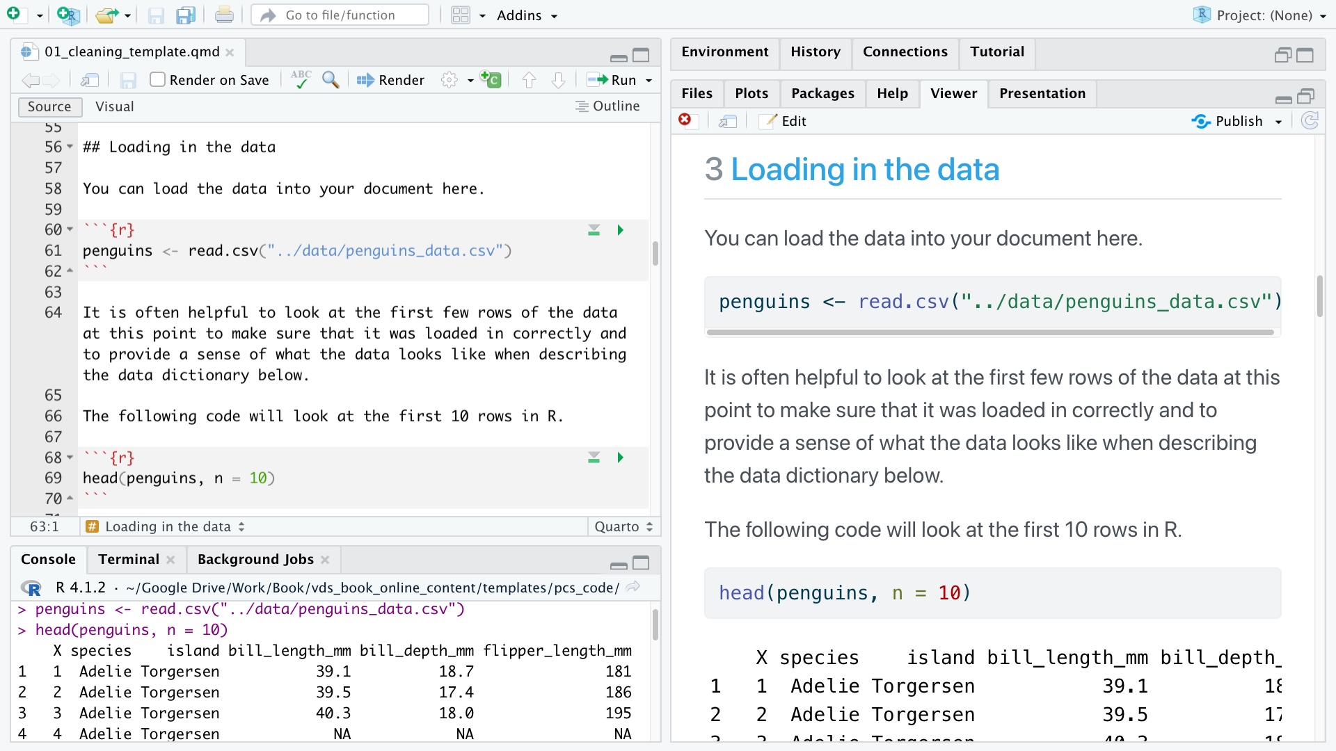
An example of a Quarto analysis document is shown in the top-left pane of the RStudio IDE shown in Figure 3.1. In the Quarto document, code is contained within the code chunks (that are surrounded by three backticks), and we are also manually running the code line-by-line in the console in the bottom-left pane. The rendered HTML version of the Quarto document is shown in the right pane.
In our recommended project structure, the dslc_documentation/ folder contains a Quarto (or Jupyter Notebook) file with the code and documentation for each relevant stage of the DSLC. For instance, the file (01_cleaning.qmd) contains the code and explanations for the data cleaning and preprocessing stage of the DSLC, and the file (02_eda.qmd) contains the code and explanations for the EDA of the DSLC. Each quarto or notebook file name is prefixed with a number designed to indicate the order in which each file should be run/read (these numeric prefixes don’t need to match the DSLC stage numbers themselves).
Reusable functions (such as data cleaning and preprocessing functions) that will be used across multiple Quarto/Jupyter Notebook files can be stored as .R (R) or .py (Python) files in the functions/ subfolder of the top-level dslc_documentation/ folder.
For real-world scientific research projects, researchers are encouraged to create an additional detailed documentation file based on the example PCS documentation template, which can be found online at https://yu-group.github.io/vdocs/PCSDoc-Template.html. This PCS documentation serves as a detailed, code-free summary of the entire project, ranging from problem formulation, data collection, and accessing the data, to the data cleaning procedure implemented (including the judgment calls made), the analyses that were conducted, the results that were obtained, and the PCS evaluations of these results. A major role of the PCS documentation is to provide a summary of the domain knowledge relevant to each stage of the DSLC, and it serves as a record of the critical thinking arguments made throughout the entire DSLC. Note that we won’t be providing complete PCS documentation for the projects in this book (the dslc_documentation/ files serve as sufficient documentation).
3.3 Reproducibility
We have used the term “reproducibility” multiple times so far in this chapter, but we have yet to formally define it. Let’s introduce the concept of reproducibility with a cautionary tale.
In 2010, Carmen Reinhart and Kenneth Rogoff, a pair of Harvard economists famous for their work on the history of financial crises, published a study called “Growth in the Time of Debt” (Rogoff and Reinhart 2010), in which they presented an analysis that showed that increasing government debt corresponding to more than 90 percent of gross domestic product (GDP) is associated with a notable decrease in economic growth. That is, the more money a government borrows (e.g., to help fund its economy during a recession), the slower its economy tends to grow. The goal of their study was to use historical economic data to make decisions about today’s economy.
Reinhart and Rogoff’s finding that increasing debt to more than 90 percent of GDP is not a good approach to dealing with times of economic difficulty quickly became a key selling point across the global economic platform for those who argued for austerity, a strategy in which governments favor lowering living standards (to save money) in times of economic difficulty rather than increasing debt (to get more money) (Blyth 2013).
However, three years after these findings began to have a widespread impact on the global economic stage, Thomas Herndon, a PhD student from the University of Massachusetts Amherst, tried to reproduce their results and couldn’t (Herndon, Ash, and Pollin 2014). In fact, together with Professors Michael Ash and Robert Pollin, he found the exact opposite result! According to Herndon et al., Reinhart and Rogoff’s original study was plagued with issues that stemmed from a lack of testing, Excel coding errors (e.g., Reinhart and Rogoff’s analysis excluded three data points from New Zealand), and insufficient documentation of the analytic process. As a result, Reinhart and Rogoff’s study was deemed by Herndon to be unreproducible.
Reinhart and Rogoff’s study is not special in this regard. A notable study (Camerer et al. 2018) tried to replicate 21 systematically selected experimental studies in the social sciences that were published in the prominent Nature and Science journals between 2010 and 2015. However, even though these articles were peer-reviewed and featured in top research journals, the researchers were able to computationally reproduce the results reported in only two-thirds of the studies. Another study, the Reproducibility Project (Open Science Collaboration 2015), tried to reproduce the results from 100 papers published in the field of psychology and was able to reproduce only around one-third of the results. This phenomenon is being called the “reproducibility crisis” in Science (Begley and Ioannidis 2015; Baker 2016).
3.3.1 Defining Reproducibility
The term reproducible has different meanings for different people, but reproducibility is generally intended as a proxy for trustworthiness. In data science, probably the most common definition says that a data-driven result is considered reproducible if you (or anyone else with the appropriate skills) can easily regenerate your results by rerunning the original code that produced it. However, results that are considered reproducible by this definition can certainly still be wrong. If your code contains mistakes (bugs) but it still runs, then you will reproduce the same wrong results every time you run it. We thus consider this definition to correspond to a fairly weak form of reproducibility. (That said, even this weakest form of reproducibility can be hard to achieve, so it is a good starting point.)
In traditional scientific research, the term “reproducible” is more likely to mean that another research group has collected its own data, conducted its own analysis, and arrived at the same conclusion as the original study. This definition involves a lot more work than the previous one, but it also offers substantially stronger evidence of the trustworthiness of the results.
Rather than trying to define specific terms for each type of reproducibility (many people have tried to do this, resulting in a jumble of inconsistent terminology—for example, Stark (2018) and Goodman, Fanelli, and Ioannidis (2016)), we will instead view several types of reproducibility in the context of the PCS framework (in increasing order of the strength of the evidence of trustworthiness that is provided):
The version of reproducibility (popular in data science) that involves demonstrating that the results can be regenerated by rerunning the original code on the same data on the same computer can be thought of as demonstrating the stability of the results to the particular instance of running the code. A slightly stronger version requires that you can rerun the original code on a different computer. This type of reproducibility provides fairly weak evidence of the trustworthiness of the results.
The example of Herndon trying to reproduce Reinhart and Rogoff’s results involved trying to reproduce the results using the same data but new code4 written by a different person. This is an example of reproducibility that corresponds to the stability of the results to the particular code that was written and to the particular person who conducted the analysis. This type of reproducibility provides stronger evidence of the trustworthiness of the results than the previous example.
The strongest examples of reproducibility involve an entirely independent team reproducing a result by collecting entirely new data and writing their own code to conduct their own analysis. This can be thought of as both demonstrating the predictability of the results (since it involves demonstrating that the results reemerge in entirely new data) as well as the stability of the results to the underlying data that was collected, to the code that was written, and to the person who wrote the analysis.
Unfortunately, you will rarely have the resources to demonstrate that your results satisfy the strongest forms of reproducibility, but we encourage you to demonstrate as many forms of reproducibility as you have the resources to accomplish. However, be warned that while achieving even this weakest form of reproducibility might seem easy, it is not. If the order in which the code was run to generate the results is not obvious, if there were pieces of code that were run but not saved (e.g., they were run directly in the console or the code was later deleted), or if the results were computed using a particularly old version of R or Python, then the results could look very different (or may not even be computable) when you or someone else try to rerun your code pipeline at a later date.
3.3.2 Tips and Tricks for Reproducibility
To maximize the chance that your results will be reproducible (in the minimal sense of obtaining consistent results every time you rerun your code), we offer the following tips:
Avoid handling raw data or doing manual modifications. If you made manual modifications to the data file (e.g., deleting some lines of text in the raw data file), but you didn’t clearly describe how and why you did this, it is highly likely that someone else who tries to reproduce your results from the raw data won’t know to conduct this step (or will conduct it incorrectly), which might result in their downstream results differing from yours. If it is absolutely necessary to make manual modifications to your data, you should clearly document what you did.
Regularly rerun your code from start to finish in a fresh R/Python session. This helps catch bugs in your code early.
Tidy up your code files. It is easy to find yourself with a jumble of messy code that doesn’t work when you run it all in order. While it is highly likely that your code and analysis will start messy—especially if you are new to coding—you are encouraged to go back over it and rewrite your code so that it is clearer and more efficient. Be sure to keep a record of all the analyses that you conducted, even if they ended up being dead ends (Stoudt, Vásquez, and Martinez 2021).
Use version control (e.g., Git). A good way of keeping a record of old code is to use version control (e.g., using Git and GitHub, which will be introduced in Section 3.4.1). The nice thing about version control is that if you “committed” (i.e., took a snapshot of) some piece of code and then later deleted or modified it, you can always retrieve it in the future if you change your mind since it will exist forever in the history of your repository. Hosting your project on GitHub is also an excellent way of showcasing your data science skills and fostering collaboration.
Document everything. Since people should be able to understand the analysis that you conducted, and the reasons why you did what you did, documentation is an incredibly important part of conducting reproducible analysis. Documentation comes in many forms, including code comments, the text you write within your Quarto/Jupyter Notebook analysis files, your README files, and if you are conducting a complex research project, perhaps in your PCS documentation as well.
Use up-to-date software. Make sure that you update R/Python and your add-on libraries every few months. This won’t necessarily happen automatically, so if you’re not careful, one day you will wake up and realize that you are using a version of R that is five years out of date and wonder why the new package that you’ve just installed doesn’t work.
3.4 Tools for Collaboration
Since most data science projects involve a team of people working together, often on the same files, it is important to have a system in place for collaborating effectively.
When it comes to producing documentation, reports, or research papers, many software applications can help teams work together simultaneously (rather than emailing different versions of reports back and forth). Google Docs allows simultaneous collaboration on notes and reports, and Overleaf lets you collaborate on LaTeX documents. Google Colab enables collaboration in a Jupyter Notebook. However, arguably the most important place where collaboration in data science takes place is on GitHub.
Unfortunately, GitHub has a bit of a technical learning curve and is not particularly accessible for nontechnical team members (although they will be able to view the files on GitHub, they may find it hard to modify them).
3.4.1 Git and GitHub
Git is a piece of software that was developed for conducting version control. Its primary task is to keep track of changes that you make to your files locally on your computer without having to save multiple versions. However, it was the advent of the online service GitHub,5 allowing for the hosting of a “remote” Git repository (“repository” is a fancy way of saying “project folder”) online that turned Git into such a powerful tool for both collaboration and version control. GitHub has fostered a global community in which data scientists and software engineers alike can connect, collaborate, and share code, analyses, and ideas. Most R and Python packages are open source as a result of being hosted publicly on GitHub, allowing anyone to fix bugs and contribute features (these contributions must be accepted by the owner of the code). Multiple people can have access to the same repository via GitHub, which contains not only the most recent versions of each file that has been “pushed” (uploaded) but also contains a record of every change that has ever been “committed” to each file. This process is a lot more sophisticated than clunky alternatives such as emailing multiple versions of code files back and forth, but this sophistication comes at the cost of a steep learning curve.
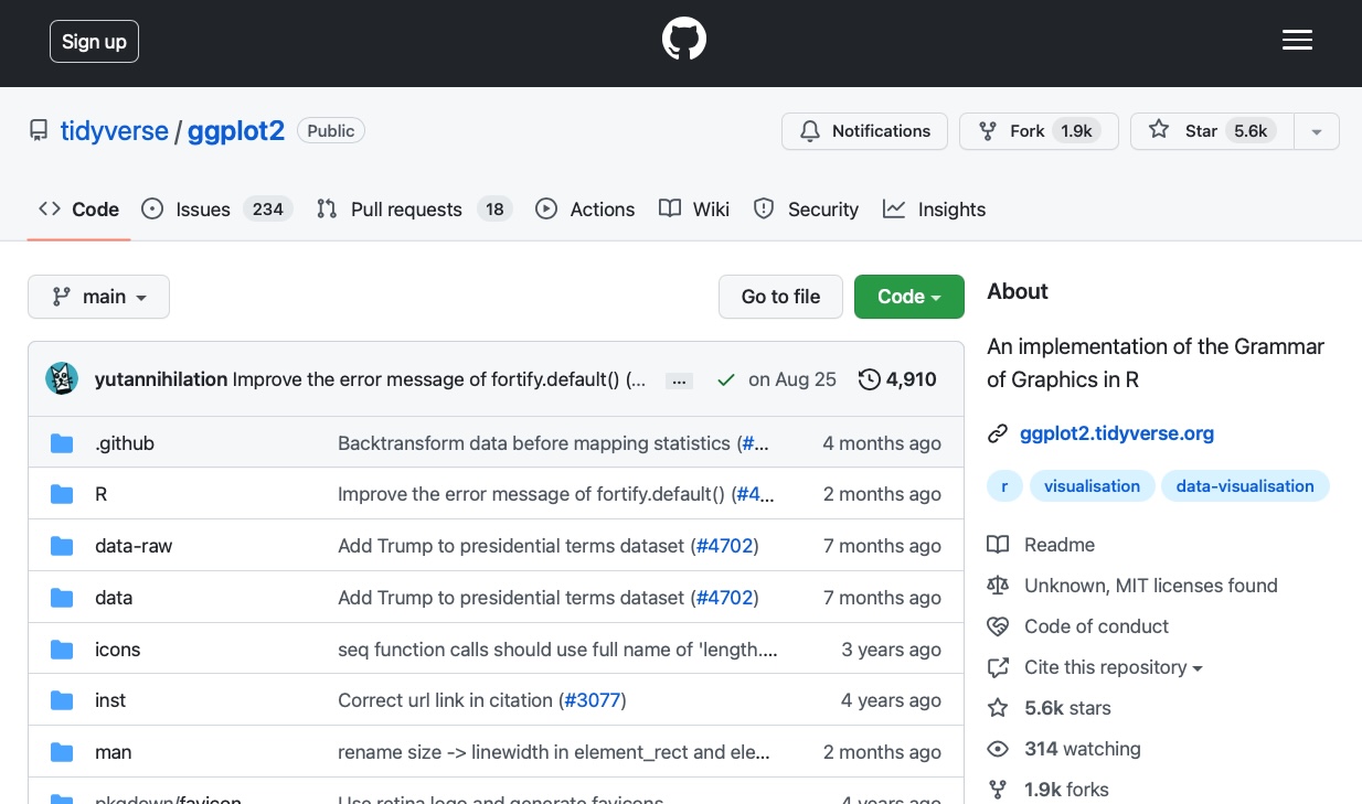
Figure 3.2 shows an example of a Git repository hosted on GitHub. This repository is for the widely used ggplot2 R package, which is a part of the tidyverse suite of packages. Anyone can “fork” this repository (create a personal version of the repository on your own GitHub account) and/or “clone” it (download it to your local machine, such as your laptop), make changes, and, if desired, submit a “pull request” which, if accepted by the repository owner, will be incorporated into the main public version of the repository.
While using Git and GitHub is not strictly mandatory for progressing through this book, if you’re hoping to eventually get a job as a data scientist, Git and GitHub will be important to know. Moreover, GitHub can be used as a portfolio to showcase your projects and present some real evidence of your skills!
For further information on Git and GitHub, some additional resources include Roger Dudler’s website “Git—the simple guide”; the Udacity course “Version Control with Git,” created by Google, AT&T, and Lyft and led by Caroline Buckey and Sarah Spikes; and the Git and GitHub notes from Software Carpentry.
To practice your Git and GitHub skills, we recommend that you create a unique GitHub repository for each of the projects that you complete in this book and use GitHub to share your analysis with the world so that your GitHub account can serve as a portfolio for showcasing your data analysis talents. As a reminder, the code for each project in this book can be found on the GitHub repository.
Exercises
True or False Exercises
For each question, specify whether the answer is true or false (briefly justify your answers).
Your
dslc_documentationfiles can contain code.It is OK to modify your original raw data file if you document the edits that you made.
It is bad practice to rerun the code that cleans your data.
R is better than Python for data science.
The term “reproducibility” is defined as being able to reproduce the same results on alternative data.
The “reproducibility crisis” is a problem unique to data science, and is not an issue in traditional scientific fields.
A good technique for increasing the reproducibility of your results (in the context of ensuring that you get the same results every time you run it) is to rerun your code from scratch often.
If someone else cannot reproduce your results (based on any definition of reproducibility), then your results must be wrong.
If someone else manages to reproduce your results (using their own independent data and by conducting their own analyses), then this proves that your results are correct.
Conceptual Exercises
What is the purpose of the
dslc_documentation/folder in our recommended project structure?Describe two techniques that help you to write clear, concise, and reusable code.
How would you frame the reproducibility analysis that Herndon and his collaborators conducted in their reevaluation of Reinhart and Rogoff’s results as a stability analysis?
One form of reproducibility evaluation involves rewriting your own code from scratch.
How would you frame this as a stability analysis?
Does this approach provide stronger or weaker evidence of trustworthiness than the approach used by Herndon?
Coding Exercises
The following exercises are designed to help you get set up with Git and GitHub for this book, but they are not a substitute for a thorough GitHub tutorial. If you have trouble with these exercises, we recommend consulting some of the additional Git/GitHub resources that are listed in this chapter. These exercises assume that you know what we mean by “the terminal,” and that you have some basic knowledge of how to use it.
Download and install Git from https://git-scm.com/downloads.
Set up a GitHub account at https://github.com/. Note that you will need to set up a Personal Access Token (PAT) on GitHub to use as a password in order to connect your local Git repositories to your remote GitHub repositories.
This exercise walks you through cloning the Veridical Data Science GitHub repository, which can be found at https://github.com/Yu-Group/vds-book-supplementary, to create a local version of it on your computer.
Navigate in your terminal (using
cd) to where you want the veridical data science folder that you’re about to download to be saved on your computer.Type:
git clone https://github.com/Yu-Group/vds-book-supplementaryin your terminal (you’ll need to be connected to the internet). This will download the files from the GitHub repository into the local directory on your computer.
This exercise involves creating a remote GitHub repository online and a local Git repository on your computer and linking them together (setting the online repository as the “remote origin” of the local repository). This will allow you to “push” and “pull” (sync) file changes.
Create a local
first_projectfolder on your computer. In your terminal, create a local folder on your computer calledfirst_project(mkdir first_project) and navigate into it (cd first_project).Create a
First-Projectremote repository online on GitHub. On the GitHub website, make sure that you are logged in and navigate to https://github.com/new to create your first repository on GitHub calledFirst-Project(no need to change any settings). Don’t close the window after you hit “Create Repository,” since you will need to copy the code that is printed beneath “… or create a new repository on the command line!”Turn your local
first_projectfolder into a Git repository and connect it to yourFirst-Projectremote repository on GitHub. In the terminal on your computer, paste the code that you copied from underneath the text “… or create a new repository on the command line”, highlighted in the following image. (Note that if you’re manually copying from this image, you will need to replacerlbarterwith your own GitHub username.)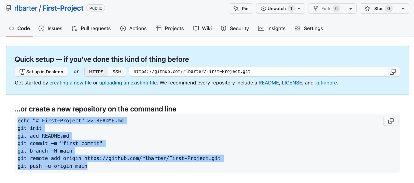
Add a file to a local Git repository and upload it to the remote GitHub repo. In the terminal on your computer, create a text document in your local
first_projectfolder calledfile.txtthat contains the text “I’m a text file” (echo "I'm a text file" >> file.txt), and confirm that the file has been created by typingls.Next, add the file to the local Git repository (
git add file.txt) and commit it (git commit -m "Created text file"). Push to your “First-Project” remote repository (git push). Confirm that the file has been uploaded to your online repository by refreshing the GitHub page containing your “First-Project” repository and verifying that it now contains the “file.txt” file, just like the image shown here (but with your username instead of “rlbarter”).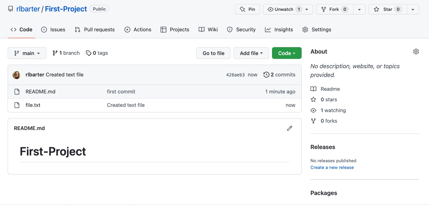
Make a change to the local file and add the change to the remote GitHub repo. Make a change to the file locally (e.g., add some more text), and then add this change (
git add file.txt), commit it (git commit -m "Edited text file"), and push it to your “First-Project” remote repository (git push).
If you managed to complete this exercise, congratulations! You’ve just set up your first Git repository, added a file, made a modification, and had those changes reflected in an online version of your repository. This is a workflow that you can use to host your own projects in an online GitHub repository (once you’ve created a repository, you can repeat the final step of the exercise to add new files and update existing files).
Note that any changes you make to the README.md file (if you add, commit, and push the changes) will be reflected on the repository home page on GitHub. If multiple people are editing the same repository you always need to pull new changes from the online repo into your local machine (git pull) before pushing your changes to avoid creating conflicts.
If you’re new to Git and GitHub, you will inevitably find yourself in unfamiliar territory with no idea what’s going on. That’s normal. We’ve all been there. Our advice is to always keep a copy of your work in these early stages (and when all else fails, delete the repository and start again). You’ll get the hang of it eventually!
References
Baker, Monya. 2016. “1,500 Scientists Lift the Lid on Reproducibility.” Nature News 533 (7604): 452–54.
Begley, C. Glenn, and John P. A Ioannidis. 2015. “Reproducibility in Science.” Circulation Research 116 (1): 116–26.
Blyth, Mark. 2013. Austerity: The History of a Dangerous Idea. Oxford University Press.
Camerer, Colin F., Anna Dreber, Felix Holzmeister, Teck-Hua Ho, Jürgen Huber, Magnus Johannesson, Michael Kirchler, et al. 2018. “Evaluating the Replicability of Social Science Experiments in Nature and Science Between 2010 and 2015.” Nature Human Behaviour 2 (9): 637–44.
Ellis, Shannon E., and Jeffrey T. Leek. 2018. “How to Share Data for Collaboration.” The American Statistician 72 (1): 53–57.
Goodman, Steven N., Daniele Fanelli, and John P. A. Ioannidis. 2016. “What Does Research Reproducibility Mean?” Science Translational Medicine 8 (341): 341.
Grolemund, Garrett, and Hadley Wickham. 2017. R for Data Science: Import, Tidy, Transform, Visualize, and Model Data. O’Reilly Media.
Herndon, Thomas, Michael Ash, and Robert Pollin. 2014. “Does High Public Debt Consistently Stifle Economic Growth? A Critique of Reinhart and Rogoff.” Cambridge Journal of Economics 38 (2): 257–79.
McKinney, Wes. 2017. Python for Data Analysis: Data Wrangling with Pandas, NumPy, and IPython. O’Reilly Media, Inc.
Open Science Collaboration, Multiple Authors. 2015. “Estimating the Reproducibility of Psychological Science.” Science 349 (6251).
Rogoff, Kenneth, and Carmen M. Reinhart. 2010. “Growth in a Time of Debt.” American Economic Review: Papers & Proceedings 100 (100): 573–78.
Stark, Philip B. 2018. “Before Reproducibility Must Come Preproducibility.” Nature 557 (7707): 613.
Stoudt, Sara, Váleri N. Vásquez, and Ciera C. Martinez. 2021. “Principles for Data Analysis Workflows.” PLOS Computational Biology 17 (3): e1008770.
RStudio, the company, changed its name to Posit in 2022, but the IDE is still called RStudio (for now, at least).↩︎
Quarto is a more flexible and customizable version of R Markdown. We use Quarto for the projects in this book, but you can easily use R Markdown files instead.↩︎
You can also use Quarto for Python, but Quarto is less common than Jupyter Notebooks for Python.↩︎
This example involved conducting an analysis within Excel, so we hesitate to use the word “code” here.↩︎
Alternatives to GitHub include GitLab and Bitbucket.↩︎