8 An Introduction to Prediction Problems
This is a pre-release of the Open Access web version of Veridical Data Science. A print version of this book will be published by MIT Press in late 2024. This work and associated materials are subject to a Creative Commons CC-BY-NC-ND license.
So far in this book, our analyses have primarily focused on understanding the underlying structure of our data and summarizing the patterns and relationships it contains. In part III of this book, we will shift gears, turning our attention to prediction problems (Box 8.1), a major topic in both traditional statistics and machine learning (ML).
Predictions play a fundamental role in our everyday decision making processes. For example, every time we go to work, we decide when to leave the house based on a prediction of how long it will take to get there. Every time we plan a dinner party, we base our decision about how much food to buy on the number of people that we predict will turn up (and how much food we expect them to eat). These “everyday” predictions that we make are typically based on cognitive data that we have mentally collected from our own past experiences.
With the increasing digitization of our society, our everyday predictions are increasingly being influenced by computational engines (for example, these days, we typically rely on Google Maps in conjunction with our own past experiences to tell us when to leave the house). Data-driven predictions permeate our society, underlying the ads that we see (based on what a tech company predicts that we will purchase), the amount that we pay for our car insurance (based on our insurance company’s prediction of our risk of having a car accident or experiencing a car break-in), and so much more.
Data-driven predictions are typically based on algorithms that quantify the relationships between a response variable that we are interested in predicting and the relevant predictor variables (often called the predictors, predictive features, attributes, or covariates).
Suppose that a company wants to predict its revenue over the next financial quarter (the unobserved future response variable of interest) by quantifying the relationship between historical revenue (a previously observed response) and the company’s spending, product sales, and stock prices (the predictive features). If revenue (the response) tends to be higher during quarters when stock prices (a predictor) are higher, and this relationship continues to hold in future data (i.e., if the relationship is predictable), then it could be used to predict the revenue in future quarters based on observed stock prices. Assuming that the resulting predictions are accurate, they could then be used to make real-world decisions. For instance, if the algorithm predicts that the next quarter’s revenue will be lower than anticipated, the company could use this information to prepare for the lower revenue (e.g., by reducing hiring or increasing the price of their product).
Note, however, that evidence of a predictive relationship between a response variable and a predictive feature does not imply a causal relationship. Just because the company’s stock prices are predictive of revenue, this doesn’t necessarily mean that increasing the stock prices (e.g., by buying back stocks) will improve the revenue.
Predictive algorithms (Box 8.2) quantify the relationship between a response variable of interest and the predictive features using existing/observed data. Specifically, they work by combining the values of the predictive features in a way such that the resulting combination—the predicted response—resembles the observed response variable as closely as possible.
In this book, the primary predictive algorithms that you will encounter are the Least Squares (LS) algorithm (as well as several variations of the LS algorithm), the logistic regression algorithm, and decision tree-based algorithms such as the Random Forest (RF) algorithm. Note that we will not be covering neural networks in this book. Additional ML resources include “The Elements of Statistical Learning” (Hastie, Friedman, and Tibshirani 2001) and the more accessible “An Introduction to Statistical Learning” (James et al. 2013).
Although predictive algorithms have been around much longer than the field of ML itself, predictive algorithms are often referred to as “machine learning” (ML) algorithms. While the term “machine learning” (ML) is often attached to prediction problems, it is actually an umbrella term for algorithms that are used to solve a range of problems (and is considered to be a part of both modern statistics and computer science). The two main types of ML problems that we discuss in this book are
Unsupervised learning: Summarizing the relationships in the data when there is no response variable. Examples include principal component analysis and clustering.
Supervised learning: Summarizing the relationships in the data with a focus on a response variable of interest whose value is observed in current/past data but is not known for future data. Examples include the prediction problems that we will be discussing throughout the rest of this book.
There are also several other types of ML problems, such as reinforcement learning, which we don’t cover in this book. See Sutton and Barto (2018) for a reference.
The rest of this chapter will define some of the prerequisite terminology and ideas for prediction problems and introduce the data project that we will be working with over the next few chapters.
8.1 Connecting the Past, Present, and Future for Prediction Problems
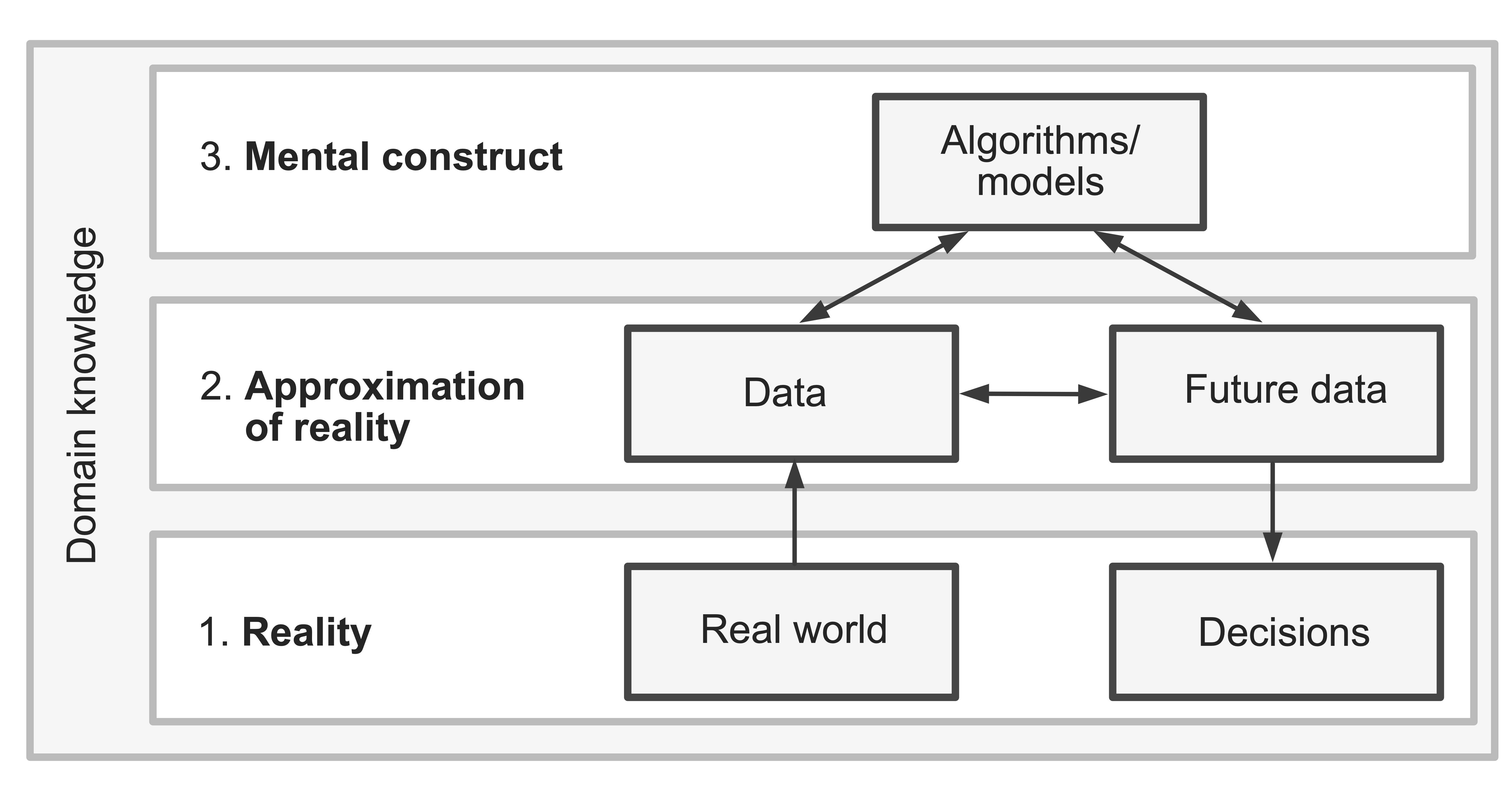
As we move into the domain of prediction problems in which our focus is applying predictive algorithms to future data to help us make real-world decisions, let’s pause to revisit the three realms shown in Figure 8.1. Recall that the three realms remind us that our data represents an approximation of reality (rather than reality itself), and the algorithms (predictive or otherwise) that we train are just mental constructs that we apply to our data.
However, even if we can use domain knowledge to provide evidence that our current data is a good approximation of reality, and we can show that the predictive fits that we produce are in line with both the data and the domain problem, we need to pay particular attention to the link between the current and future data.
That the future and present reality (and data) will be similar to one another isn’t necessarily obvious. The world around us is constantly evolving, causing the underlying trends and real-world physical relationships to change. If a prediction algorithm is accurately capturing trends contained within the current data, but the underlying real-world trends change (e.g., a global pandemic disrupts the entire global economy), then the algorithm might not be able to yield accurate predictions for future data (even if the future data was collected using the same data collection mechanism as the current data).
The assumption that the relevant underlying patterns and trends remain the same over time is major, which is why it is so important to evaluate our algorithms on withheld data that is a good representation of the future data to which they will be applied (or, better yet, on actual future data). Unfortunately, it is not always obvious when the underlying real-world patterns and trends have changed. Whenever possible, it is a good idea to compare the future data to the current data and to use domain knowledge to identify whether the underlying patterns, trends, and relationships have changed over time to determine whether our algorithms are relevant to the real-world scenarios to which we intend to apply them.
We are assuming here that our predictive algorithms will always be applied in a similar (future) context to that in which it was trained. In practice, however, it is becoming more and more common for predictive algorithms trained in one context to later be applied in an entirely different context.1 For example, imagine that a medical device company has developed a new pulse oximeter (a device that is placed on the patient’s fingertip to measure blood oxygen saturation levels using light). Since the company was located in Santa Barbara County in California (whose population is 75 percent white), the device was tested and calibrated primarily using a cohort of predominantly white people. If, however, the hospitals and physicians that purchase the pulse oximeters use them on a much more racially diverse set of patients, then they are inadvertently using the device in a context that is different from that in which it was developed. Since the device was optimized for a population of predominantly white people, the result might be that the pulse oximeters are less accurate for patients with darker skin tones, potentially exacerbating racial health outcome inequalities. Unfortunately, several real-world studies have indeed found that pulse oximeters tend to overestimate blood oxygen saturation levels in Black, Asian, and Hispanic patients compared to white patients, and as a result, people of color often experience greater delays in receiving lifesaving treatments (Fawzy et al. 2022; Sjoding et al. 2020).
This is not to say that you should never apply algorithms to settings that they were not trained in, but rather that it is critical to communicate the data context in which your algorithms were trained and to ensure that whenever it is being used in a new setting, that you (or whoever is using it) explicitly demonstrate that it works well in the new setting.
8.2 Setting up a Prediction Problem
In this section, we will discuss how to identify an appropriate response variable and ensure that you have access to relevant predictor variables for your prediction problem.
8.2.1 Defining a Response Variable
The first step in getting your prediction project off the ground is to translate your domain problem goal into a prediction problem. This involves precisely specifying what you want to predict (i.e., specifying a response variable whose value will help address your domain question). For the pulse oximeter example, the response variable is each patient’s blood oxygen level, and for the company revenue example, the response variable is the revenue for each quarter.
To train an algorithm that can predict the value of a response for future data whose response variable is unknown, you need to first have access to labeled data (Box 8.3), which is current/historical data whose response variable is known (has been observed/measured). After all, how can you learn about the relationships between the response variable and predictive features if your data doesn’t include the response variable?
For some problems, obtaining labeled data is easier than for others. If the response is always recorded in the historical data, then obtaining labeled data might just involve collecting historical data that includes the response information. However, for some prediction problems (such as predicting whether a pathology image contains a tumor from a collection of unlabeled pathology images) the data may need to be manually labeled—a process that often requires a lot of time, resources, and domain expertise!
The two most common types of response variables that you will encounter are the following2:
Binary responses that are always one of two possible values. Examples of binary responses include the results of a factory quality control test (pass/fail), whether a user will click on an advertisement on a webpage (click/not click), or whether an email is spam (spam/not spam). Binary response prediction problems are often called classification problems in traditional statistics and ML.
Continuous responses that can be an arbitrary numeric value. Examples of continuous responses include patient survival (in months), tomorrow’s maximum temperature (in degrees Fahrenheit), and a company’s annual revenue (in dollars). Continuous response prediction problems are often called regression problems in traditional statistics, but since the term “regression” is heavily associated with traditional statistical inference, data-generating assumptions, and theoretical guarantees, we won’t be using this term heavily in this book.
Some questions can be formulated with either a binary or a continuous response, based on how you ask the question. For instance, if you are working on a project whose goal is to predict the survival of melanoma patients, you could formulate the question as one that has a binary response: will the patient survive for more than six months from diagnosis (yes/no)? Or you could formulate the question with a continuous response: how long will the patient survive after their diagnosis (in months)? For some problems, converting a continuous response to a binary response (e.g., using a threshold) can simplify the prediction problem and lead to more accurate predictions. Note that some predictive algorithms can be used for predicting both continuous and binary responses, whereas others are designed specifically for continuous or binary response problems.
8.2.2 Defining Predictor Variables
Having identified and measured a suitable response variable, the next task is to ensure that the data contains appropriate predictive features. The predictive features contain the information that will be used to generate the response predictions. If you are predicting the sale price of a house (the response variable), relevant predictive features might be the size of the house, the age of the house, and the condition of the house. Domain knowledge will typically be used to determine which features may be important predictors of the response.
For a variable to be an appropriate predictive feature, its value needs to be available (measured/observed) even when the response variable is not, and it should not depend on the response variable itself. For instance, suppose that you are using historical housing sale data to predict sale prices, and this data contains information on the amount of tax paid on each sale. Although this information would likely be very predictive of the house’s sale price, it is itself determined by the sale price of the house and its value has not been observed for future houses that have not yet been sold. This tax variable is thus not an appropriate predictive feature.
Note that row identifier variables or ID variables are also not appropriate predictive features. Be sure to remember to remove inappropriate predictive features during preprocessing!
8.2.3 Quantity versus Quality
While it is generally argued that more data will lead to better predictions, this is not always the case. Having more data (in terms of either more observations or more predictive features, or both) will lead to more accurate predictions only if the additional observations and predictive features are of good quality and provide additional relevant information for predicting the response. For instance, if you are simply adding more observations (rows) that are essentially identical to the existing observational units in the data, or are adding more predictive features (columns) that have nothing to do with the response, then you are unlikely to see much improvement in your predictive performance (and you may even unintentionally introduce numerical instability into your predictive algorithm). When it comes to collecting additional information, we recommend focusing on quality over quantity. You will generally be better off having a smaller but more diverse dataset with a few highly relevant features (e.g., chosen using domain knowledge) than a larger but more uniform dataset with a large number of only vaguely relevant features.
8.3 PCS and Evaluating Prediction Algorithms
As with all other analyses we have conducted in this book, any predictive results that you produce need to be evaluated in the context of the PCS framework. Recall that the purpose of the PCS framework is to provide evidence of the trustworthiness of your computationally derived results by demonstrating that they are predictable (i.e., reemerge in new scenarios, especially those that resemble the context in which they will be used for decision making) and stable (i.e., are not overly dependent on the specific data that we used and the judgment calls that were made throughout the DSLC). While the PCS principles for prediction problems are similar to those for the exploratory, dimensionality reduction, and clustering problems that we have seen so far, it is worth taking a moment to highlight how the PCS framework will be used in the context of prediction problems.
8.3.1 Predictability
The most common way to demonstrate the predictability of the results of a predictive algorithm is to show that the algorithm generates accurate response predictions for data that resembles the future data that the algorithm will be applied to in practice. For instance, if you will be using your algorithm to predict the unknown response for future data points (such as to predict the sale price of future houses for sale in the same city or the prognosis for future patients from the same hospital as the original data), then you should try to evaluate it on data that was collected after the original data that was used to train it. Similarly, if you will be using the algorithm to predict the unknown response for data points collected from a different source (such as to predict the sale price of houses in a neighboring city or the prognosis for patients in a different hospital), then you should evaluate it on data that comes from a different source than the original data used to train it.
The problem is that when it comes to evaluating prediction algorithms (e.g., computing the accuracy of response predictions), the data that you use to evaluate your predictions need to be labeled (which means that the response value needs to have been measured and recorded in the data). This is, unfortunately, often not the case for actual future data or external data. For instance, we don’t know how much the houses that are currently (or will soon be) on the market will sell for, nor do we know what the eventual outcomes for newly diagnosed patients will be. That is, most future/external data has not yet been labeled.
8.3.1.1 Training, Validation, and Test Datasets
When we don’t have access to additional future or external labeled data similar to that to which we will be applying our algorithm, we will often instead withhold some validation data from our current observed labeled data to use for evaluation.
Although we advocated splitting the data three ways into a training set, validation set, and test set earlier in this book, you may have noticed that we have yet to use the test dataset. In prediction problems, the validation data is often used to filter out poorly performing algorithms and decide on the “final” version of the predictions (which may involve comparing various algorithms to choose the best-performing one, creating an ensemble of several of the best-performing algorithms, or even producing an interval of predictions created from the best-performing algorithms). However, this means that information from your validation dataset has now been used in the process of generating your final prediction results, and thus it can no longer be used to provide a reasonable assessment of how well your final predictions (or ensemble or interval of predictions) will perform on future or external data (recall the concept of “data leakage” from Chapter 1). This is where the test dataset comes in! Since the test dataset has not yet been used to choose the final predictions, it can still act as a reasonable surrogate of future or external data.
Recall that your data should be split into training, validation, and test datasets in such a way that the validation and test datasets reflect the future, new, or external data to which you intend to apply your results, such as using a time-based, group-based, or random split (for a recap, see Section 1.3.1.1 in Chapter 1).
8.3.1.2 Reality Checks for Prediction Problems
Additional evidence of predictability can be obtained from conducting reality checks by identifying whether your algorithm is uncovering known or expected relationships. Since many predictive algorithms involve quantifying relationships between predictor and response variables (which may or may not be capturing the actual mechanism of the relationship), if your predictive algorithm appears to be capturing known or plausible relationships (according to domain experts and/or domain knowledge), then you can use this as evidence that the algorithm is capturing predictable information.
However, to avoid confirmation bias, when presenting such results to domain experts, it is a good idea to show them multiple possible versions of the captured relationships, only one of which will be the actual version produced by your algorithm. If the domain expert chooses the “real” version from among the collection of results shown to them, then you can feel more confident that the relationships that you have captured seem reasonable.
8.3.2 Stability
Just as with other techniques we have introduced in this book, the stability of your response predictions can be assessed by training multiple versions of the predictive algorithm under different data and judgment call perturbations, and investigating the extent to which the predictions and predictive performance change.
8.4 The Ames House Price Prediction Project
In part III of this book, we will introduce two data projects. The first, the Ames house price prediction project, has a continuous response, and our goal is to predict the sale price of houses in the city of Ames, which is a college town in the state of Iowa. The second, the online purchase prediction project, has a binary response, and our goal is to predict which user sessions on an e-commerce website will make a purchase. Since we will be starting with continuous response prediction problems, we will introduce the data for the Ames house price prediction project here and we will introduce the online purchase prediction project in Chapter 11 when we discuss binary prediction problems.
For the Ames house price project, let’s imagine that we’re looking to buy a house in Ames, but we want to focus our housing search attention on houses that are likely to sell within our predetermined price range. Our goal for this project will be to develop an algorithm for predicting the sale prices of houses for sale in Ames.
8.4.1 Data Source
For this project, we will use data that contains information on houses sold in Ames from 2006 to 2010 that has been provided by De Cock (2011). According to the paper that he wrote about this dataset, De Cock obtained this data directly from the Ames City Assessor’s Office.
The response variable is the sale price of the houses, which is a continuous numeric variable. The dataset contains around 80 predictor variables (columns) measured for each of the 2,930 houses (rows) that were sold in Ames between 2006 and 2010. Table 8.1 shows the data from the sale price response variable and five of the predictor variables for 10 randomly selected houses from the raw dataset.
| SalePrice | Neighborhood | Lot Config | Gr Liv Area | Overall Qual | Kitchen Qual |
|---|---|---|---|---|---|
| 215000 | Gilbert | Inside | 1959 | 7 | Gd |
| 137000 | NAmes | Inside | 1728 | 5 | TA |
| 145250 | NAmes | Inside | 1383 | 6 | TA |
| 124000 | NAmes | Inside | 1025 | 5 | TA |
| 129000 | Sawyer | Inside | 894 | 5 | TA |
| 192000 | ClearCr | Inside | 2022 | 7 | TA |
| 211000 | CollgCr | Corner | 1992 | 7 | Gd |
| 137500 | Edwards | Inside | 1181 | 4 | TA |
| 138887 | Crawfor | Inside | 1784 | 5 | TA |
| 172500 | Timber | Inside | 1442 | 5 | TA |
Although the data came from a reputable source, the Ames City Assessor’s Office, we have very limited information about how the measurements in the data were recorded. Was there a single assessor who visited every house and took the measurements, or were there multiple assessors? Were some variables already available in a preexisting database, or was every variable measured anew when a house was listed for sale? Was the data entered directly into a database, or was it first recorded on a physical form and then copied into a spreadsheet? The answer to these questions is: We don’t know (and to find out, we would likely need to get in touch with someone from the Assessor’s Office and hope that the people who curated this data still work there and we can identify them). That said, since we are conducting this project for educational purposes, we feel OK not knowing (but if this were a real project with real-world consequences, we would encourage making a reasonable effort to answer these questions).
8.4.2 The Ames Housing Market: Past versus Future
Let’s take a moment to consider the connections across the three realms (Figure 8.1) for the Ames house price project. Specifically, let’s focus on whether there is a connection between the current data provided by De Cock and the future data to which we would be applying our algorithm.
Suppose that our goal is to buy a house in Ames in the near future (which, at the time of writing, is the year 2024). However, De Cock’s dataset was collected between 2006 and 2010. Given that it is now more than a decade after this data was originally collected, it unfortunately seems unlikely that this data would resemble the housing market in Ames today. From our own domain knowledge, we know that housing prices have changed dramatically over the past few decades, so even without doing any research, we can already tell that the assumption that this dataset will be relevant to the Ames housing market of today is dubious.
Let’s back this up with some data. A quick search led us to some additional Ames house price trend data, specifically, “a smoothed, seasonally adjusted measure of the typical home value” provided publicly by Zillow. Figure 8.2 shows the Zillow Ames house price trends from 2005 and 2020, with the time period covered by De Cock’s house price data highlighted in gray. It is disturbingly clear that the sale prices during the time period that De Cock’s data covers are very different from the sale prices of a decade later: house prices in Ames grew from an average of around $190,000 in 2010 to an average of around $240,000 in 2020. Any predictive algorithm that we build using data from between 2006 and 2010 is going to vastly underpredict the sale price for houses today. It therefore seems that there is not a strong connection between the current and future data for this project.

Unfortunately, there isn’t a more recent publicly available Ames housing dataset that includes information on the predictive features of houses for sale (the Zillow data only contained aggregate sale prices, but did not contain the individual house-level predictive features). Recall that De Cock originally collected this data by getting in touch directly with the Ames City Assessor’s Office. Since we do not want to bother the Assessor’s Office for this educational example (and even if we did, we might not find the information we’re looking for), and since we won’t be applying whatever algorithm we create in the real world, we will make a compromise. We’re going to pretend that we live in 2011 (the year after De Cock’s dataset ends) as we conduct this project.
8.4.3 A Predictability Evaluation Plan
Since we don’t have access to any external housing price data that contain the same variables as De Cock’s dataset, we will split the data into training, validation, and test sets. The resulting validation and test datasets will then act as surrogates for the future data to which we would apply our predictive algorithms, which in this case represents the hypothetical 2011 Ames housing data. Since there is a time dependency in De Cock’s data (the data were collected over five years) and we would be applying our algorithms to future data, we will use the following time-based split:
The training data contains the earliest 60 percent of the data, corresponding to houses sold between January 1, 2006 and August 1, 2008 (i.e., 60 percent of the houses in the data were sold on or before August 1, 2008).
The validation data contains a randomly selected half (or the first half) of the houses sold between August 2, 2008 and July 1, 2010 (when the data ends). This corresponds to 20 percent of the data.
The test data contains the remaining houses (i.e., those not included in the validation dataset) sold between August 2, 2008 and July 1, 2010. This also corresponds to 20 percent of the data.
The training data will be used to develop several predictive algorithms, the validation data will be used to compare them and filter our poorly performing algorithms, and the test data will be used to evaluate the final algorithm.
8.4.4 Cleaning and Preprocessing the Ames Housing Dataset
Before reading this section, if you’re coding along, we suggest spending some time exploring and cleaning the Ames dataset yourself (refer back to Chapter 4). The data and our cleaning and preprocessing process for the Ames house price project can be found in the ames_houses/ folder on the supplementary GitHub repository.
Since we are only interested in residential properties, upon loading the data, we immediately excluded all 29 nonresidential properties from the data (based on the MS Zoning variable). We also excluded all 517 sales that were foreclosures, adjoining land purchases, deed reallocations, internal-family sales, and incomplete houses (based on the Sale Condition variable).
Recall that the goal of data cleaning is to ensure that the data is as unambiguous as possible and adheres to a tidy format. Some of the data cleaning steps that we implemented in the 01_cleaning.qmd (or .ipynb) file in the ames_houses/dslc_documentation/ subfolder of the supplementary GitHub repository include the following:
Converting the variable names to human-readable, lowercase, and underscore-separated variable names. For instance,
Paved Drivebecamepaved_drive, andFireplace Qubecamefireplace_quality.Replacing the seemingly erroneous 1950 entries in the
Year Remod Addvariable (the year that a remodel was added) with theYear Builtvalue (the year that the house was built).Replacing blank entries (
"") with explicit missing values (e.g.,NAin R).
Note that the data contains many categorical variables that must be converted to numeric variables during preprocessing before we apply many of the predictive algorithms that we will introduce over the next few chapters. Some of the preprocessing steps that we conducted to ready the data for training the prediction algorithms include the following:
Converting ordered categorical variables into meaningful numeric variables. For instance, the
Exter Cond(exterior condition) variable is originally coded using categorical text values:Ex(excellent),Gd(good),TA(typical/average),Fa(fair),Po(poor). We converted these levels to a numeric variable with values 5, 4, 3, 2, and 1 for each level, respectively.Removing variables that have the same value for almost all the houses, such as the
Utilitiesvariable. The threshold of the proportion of identical values above which the variable is removed is a judgment call.Removing variables for which more than 40 percent of their values are missing. This 40 percent threshold is a judgment call.
Lumping all but the 10 most common
neighborhoodvalues into an “Other” category, and then converting theneighborhoodvariable into binary (dummy/one-hot encoded) variables (we will discuss dummy variable/one-hot encoding preprocessing in Chapter 10). The number of neighborhoods to keep is a judgment call.
Multiple judgment call options for several of these preprocessing steps were included as arguments in our preprocessing function.
Table 8.2 shows one version of the cleaned and preprocessed data originally shown in Table 8.1. Due to space constraints, we only show six columns.
| sale_price | neighborhood_NAmes | neighborhood_Sawyer | lot_inside | gr_liv_area | overall_qual | kitchen_qual |
|---|---|---|---|---|---|---|
| 215000 | 0 | 0 | 1 | 1959 | 7 | 4 |
| 137000 | 1 | 0 | 1 | 1728 | 5 | 3 |
| 145250 | 1 | 0 | 1 | 1383 | 6 | 3 |
| 124000 | 1 | 0 | 1 | 1025 | 5 | 3 |
| 129000 | 0 | 1 | 1 | 894 | 5 | 3 |
| 192000 | 0 | 0 | 1 | 2022 | 7 | 3 |
| 211000 | 0 | 0 | 0 | 1992 | 7 | 4 |
| 137500 | 0 | 0 | 1 | 1181 | 4 | 3 |
| 138887 | 0 | 0 | 1 | 1784 | 5 | 3 |
| 172500 | 0 | 0 | 1 | 1442 | 5 | 3 |
8.4.5 Exploring the Ames Housing Data
In the 02_eda.qmd (or .ipynb) code/documentation file in the relevant ames_houses/dslc_documentation/ subfolder of the supplementary GitHub repository, we conducted an EDA of the Ames housing data. As an example of some of the explorations that we conducted, Figure 8.3 shows a bar chart displaying the correlation of each numeric predictor variable with the response variable (sale price). While correlation isn’t an ideal measure for variables that aren’t continuous (several of our variables are binary numeric variables that are either equal to 0 or 1), it is still a quick way to get a general sense of which variables seem to be related to the sale price. From Figure 8.3, it seems as though the quality of the house (overall_qual) and the total living area (gr_liv_area) of the house are the two features that are most highly correlated with the sale price.

To take a closer look at two of these features, Figure 8.4(a) displays boxplots comparing the distribution of the sale price response variable for each quality score value and demonstrates that the sale price tends to be higher for houses with higher “quality” scores (although notice that the relationship doesn’t look linear, but rather has a curved—perhaps even an exponential—relationship). Figure 8.4(b) displays a scatterplot that compares the living area predictive feature with the sale price response, and demonstrates that larger houses tend to have higher sale prices. These are fairly unsurprising trends (they are in line with what we would expect based on domain knowledge), but it is helpful to see that these relationships look quite strong. When training some predictive algorithms in the upcoming chapters, we will expect these features to be strong predictors of sale price.

Exercises
True or False Exercises
For each question, specify whether the answer is true or false (briefly justify your answers).
For any given domain problem, there are many ways that you could define a response variable.
Labeled data is required for training a predictive algorithm, but not for evaluating it.
Creating training, validation, and test datasets using a random split will always be appropriate, no matter the domain problem or future data scenario.
A predictor variable that has a strong predictive relationship with the response variable does not necessarily imply a causal relationship between the predictor and response.
Predictor variable, predictive feature, predictor, and covariate are all different terms used to refer to the same thing (i.e., the variables that are used to generate a prediction of a response).
Cluster membership labels can be thought of as real-world “ground truth” response labels for predictive problems.
Collecting more training data observations will always lead to algorithms that produce more accurate predictions.
Collecting additional predictor variables will always lead to more accurate predictions.
Conceptual Exercises
Imagine that you work for a search engine company and are tasked with learning about which types of user queries (i.e., phrases that users type into the search engine) result in revenue by developing an algorithm that will predict whether a particular user query will lead to an ad click.
If each observation corresponds to a user query, suggest a potential continuous response variable for this problem.
If each observation corresponds to a user query, suggest a potential binary response variable for this problem.
Suggest a few predictor variables that you could collect that might be good predictors of your (binary or continuous) response.
How would you evaluate the predictability of your algorithm’s predictions?
Suppose that you came across a (supposedly very accurate) algorithm for predicting whether it will rain in your town each day using atmospheric measurements from the previous three days (such as temperature, pressure, humidity, etc.).
If this algorithm was trained using data from one particular city in your state that is 100 miles from your town, how might you determine whether the algorithm is appropriate for use in your town?
If the algorithm was instead trained using data from your town, but it was trained using data that was collected more than 10 years ago, how might you determine whether the algorithm is appropriate for use today?
Imagine that you are tasked with developing an algorithm for predicting whether a flight will be delayed using airport flight data collected from flights to and from US airports between 2017 and 2022.
What are the observational units for this data?
Identify an appropriate response variable for this prediction problem. Note whether it is binary or continuous.
List four predictive features you think might help predict your response variable.
What is the future data you would apply this algorithm to?
If you don’t have access to any additional data, how would you split the existing data into training, validation, and test datasets to conduct a predictability evaluation?
Identifying Arctic ice cover using static satellite imagery can be a surprisingly challenging problem due to the visual similarity between cloud and ice in satellite images. Imagine that your job is to develop a computational algorithm for predicting whether each pixel of a satellite image taken over an Arctic region corresponds to cloud or ice.
Your hypothetical data consists of a single image (covering an area of 100 square kilometers). The image has been converted into a tidy rectangular format, where each row corresponds to a pixel (there are over 100,000 pixels) and the variables/features recorded for each pixel include the grayscale intensity value for the pixel, as well as some more complex features such as the radiance (the brightness detected in a given direction directed toward the sensor) recorded for several angles and wavelengths. Each pixel in the image has been labeled by an expert based on whether it corresponds to cloud or ice.
What are the observational units for this data?
Define a response variable for this prediction problem. Identify whether it is binary or continuous.
If you only have one image on which to both train and evaluate your algorithm, how would you split your pixels (which come from a single image) into training, validation, and test datasets? Hint: think about whether there is a dependence between the pixels in the image as well as the kind of data to which you would be applying the algorithm.
If your algorithm can generate accurate predictions for another similar image taken nearby, discuss whether you would feel comfortable using your algorithm trained on this data to predict the locations of cloud and ice across a range of different Arctic regions.
References
De Cock, Dean. 2011. “Ames, Iowa: Alternative to the Boston Housing Data as an End of Semester Regression Project.” Journal of Statistics Education 19 (3).
Fawzy, Ashraf, Tianshi David Wu, Kunbo Wang, Matthew L. Robinson, Jad Farha, Amanda Bradke, Sherita H. Golden, Yanxun Xu, and Brian T. Garibaldi. 2022. “Racial and Ethnic Discrepancy in Pulse Oximetry and Delayed Identification of Treatment Eligibility Among Patients with COVID-19.” JAMA Internal Medicine 182 (7): 730–38.
Hastie, Trevor, Jerome Friedman, and Robert Tibshirani. 2001. The Elements of Statistical Learning. Springer. Springer.
James, Gareth, Daniela Witten, Trevor Hastie, and Robert Tibshirani. 2013. An Introduction to Statistical Learning: With Applications in R. 1st ed. Springer.
Sjoding, Michael W., Robert P. Dickson, Theodore J. Iwashyna, Steven E. Gay, and Thomas S. Valley. 2020. “Racial Bias in Pulse Oximetry Measurement.” New England Journal of Medicine 383 (25): 2477–78.
Sutton, Richard S., and Andrew G. Barto. 2018. Reinforcement Learning: An Introduction. 2nd ed. MIT Press.